Area of Research: Diffusion of Social Phenomena
Will the Rest of the World Live Like America?
Bi-Logistic Growth
This paper first appeared in the journal Technological Forecasting and Social Change, published by Elsevier Science Inc., New York.
Introduction
Many processes in biology and other fields exhibit S-shaped growth. Often the curves are well modeled by the simple logistic growth function, first introduced by Verhulst in 1845. Although the logistic curve has often been criticized for being applied to systems where it is not appropriate, it has proved useful in modeling a wide range of phenomena. Kingsland [1] provides a thorough history of the applications of the simple logistic curve in population ecology, its successes and failures. Marchetti and colleagues at IIASA [2,3], as well as many others [4], have shown thousands of examples, mainly in socio-technical systems. Recently, Young [5] surveyed and compared growth curves used for technological forecasting, including the logistic function. Almost all the analyses and successes apply to the case of a single growth process operating in isolation. Here, I extend the analysis of logistic functions to cases where dual processes operate.
The carrying capacity of a human system is often limited by the current level of technology, which is subject to change. More generally, species can sometimes alter and expand their niche. If the carrying capacity of a system changes during a period of logistic growth, a second period of logistic growth with a different carrying capacity can superimpose on the first growth pulse. For example, cars first replaced the population of horses but then took on a further growth trajectory of their own. We call such a system with two logistic growth pulses, growing at the same time or sequentially, “Bi-logistic.” As I will show, the Bi-logistic is useful in modeling many systems that contain complex growth processes not well modeled by the simple logistic.
The plan of this paper is as follows. First, a model based on the sum of two simple logistic growth pulses is presented in order to analyze systems that exhibit Bi-logistic growth. A nonlinear least-squares algorithm is described that allows values for the model parameters to be estimated from time-series growth data. Then, model sensitivity and robustness are discussed in relation to error structure in the data. Finally, a taxonomy and examples of systems that exhibit Bi-logistic growth are discussed.
Logistic Growth
The logistic law of growth assumes that systems grow exponentially until an upper limit or “carrying capacity” inherent in the system is approached, at which point the growth rate slows and eventually saturates, producing the characteristic S-shape curve [6]. In the simple exponential growth model, the growth rate of a population, N(t), is proportional to the population
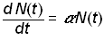
.(1)
As a consequence, there are no limits to growth; as t® ¥, N(t)® ¥. In the familiar analytic form, a is a growth rate parameter and b is a location parameter that shifts the curve horizontally but does not alter its shape:
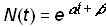
(2)
The logistic model adds to the exponential model (1) a feedback term that slows the growth rate of the system as the “carrying capacity” or saturation parameter k is reached
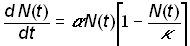
(3)
For values of N(t) << k, equation (3) closely resembles exponential growth. As the population N(t) approaches k, the feedback term causes the rate of growth to slow to zero, giving rise to the familiar symmetrical S-shaped curve. The logistic law of growth arises as a solution to equation (3)
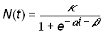
(4)
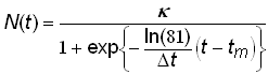
where a is a rate parameter; b is a location parameter (it shifts the function in time but does not affect the function’s shape); and k is the asymptotic value that bounds the function and therefore specifies the level at which the growth process saturates [7]. Symmetry implies that the logistic function has a point of inflection at k/2. It is convenient to define tm as the midpoint of the growth process: N(tm) = k/2. The location parameter b can be replaced by tm by defining b = -tma. It is also convenient to define a parameter Dt as the length of the time interval required for the growth process to grow from 10 to 90 percent of the saturation level k. The length of this interval (derived through simple algebra) is Dt = (ln81)/a.
An equivalent form of the standard 3-parameter logistic model (4) with parameters convenient for the analysis of historical time-series data can be defined as
.(5)
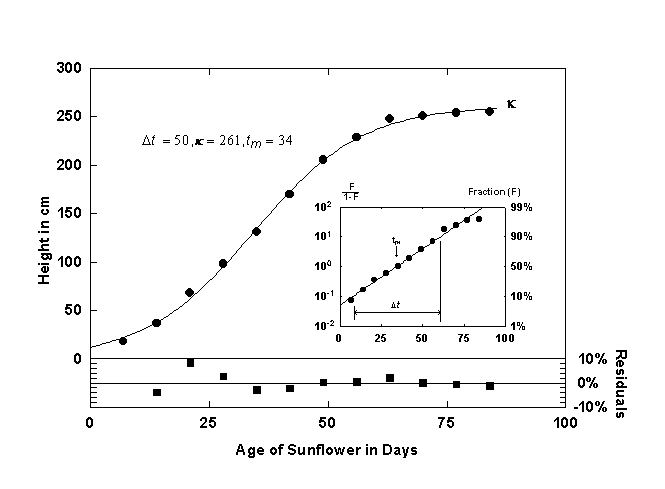
Figure 1. Growth of a sunflower fitted with a single logistic curve. The inset shows the logistic curve and the data linearized with the Fisher-Pry transform. The lower panel shows the residuals in percent deviation from the fitted curve. Source of data: [8].
Figure 1 shows the growth of a sunflower [8] and the corresponding logistic curve. The residuals (in percent deviation) are plotted in t he panel beneath the logistic curve.
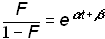
The logistic growth curve can be linearized by a change of variable (first discussed by Fisher and Pry [9]), by defining

(6)
and substituting into equation (4)
.(7)
Plotting equation 7 with a logarithmic y-axis produces a straight line, and Dt and tm can be easily read off this plot if the corresponding percents of saturation are marked. Plotting the logistic linearly also facilitates the rapid comparison to other logistic growth processes because all the curves are normalized by k. The inset of Figure 1 shows the sunflower data and the corresponding logistic curve plotted linearly. If k is known, the parameters Dt and tm can be determined by using a linear regression technique to fit a straight line through the transformed data.
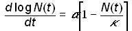
As discussed, the logistic growth model has been successfully applied to a wide range of biological and socio-technical systems. To explain why the logistic is so pervasive, Montroll [10] postulates “laws” of social dynamics modeled after Newton’s laws of particle dynamics. The first law of social dynamics states that “in the absence of any social, economic, or ecological force, the rate of change of the logarithm of a population, N(t), of an ‘organism’ is constant”,

.(8)
This is equivalent to Newton’s first law, which states that a particle in motion in the absence of any external forces will travel in a straight line with constant velocity. Equation (8) is also equivalent to exponential growth.
Montroll’s second law of social dynamics states that equation (8) is violated when a social, economic, or ecological force is applied. One of the simplest “forces” that could replace the right-hand side of equation (8) is a linear force proportional to the population:

(9)
which represents a deterrence to population growth. If g is replaced by a/k, where k is the carrying capacity, equation (8) becomes
(10)
which is equivalent to the logistic model (3). Thus, logistic growth can be viewed as a canonical form of growth for a system that is subject to forces that slow unconstrained growth. If multiple forces operate, a system can undergo more than one logistic growth pulse, as will be discussed shortly.
Bi-Logistic Growth
The standard 3-parameter form of the logistic growth model describes one period or “pulse” of growth as the system proceeds from rapid exponential growth to slow growth as the carrying capacity k is approached. Multiple growth pulses characterize many systems. In the case of a system with two well-defined serial logistic growth pulses, it is possible to split the time-series data set in two and model each set with a separate 3-parameter logistic function. This method is limited because it is often unclear exactly where to split the data set. Cases appear rare where one process ends entirely before the second begins. Problems arise in assigning values from the “overlap” period to the first or second pulse.
A superior alternative is to analyze systems that exhibit Bi-logistic growth by using the time-series data to estimate the parameters of a model comprised of the sum of two 3-parameter logistic growth pulses. The Bi-logistic growth model is then

.(11)
Selection of a method to estimate the parameters depends on the assumed distribution of the measurement errors in the data. A standard procedure is to assume that the measurement errors are independently and normally distributed with constant standard deviation. The best-fit parameters can then be found by minimizing the sum of the squares of the residuals. The residuals are defined as the difference between the time series data set (ti,yi) with m data points and the Bi-logistic model N(t)

Residuals = i = 1…m(12)
The parameter estimates can then be found by using a nonlinear regression technique to minimize the sum of the squares of the residuals
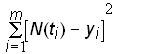
Minimize(13)
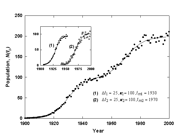
Figure 2. Example of a Bi-Logistic growth curve generated with 3% relative Gaussian error. The inset shows component growth curves.
The measurement errors of many historical data sets are unknown. Thus the common assumption that the errors are independently and normally distributed is often invalid. A least-squares method of regression can still be used to estimate parameters for these data sets, but the estimates are no longer guaranteed to be unbiased. When the measurement errors of a time series data set are unknown, as in the examples presented later in this paper, an ordinary least-squares regression technique, which gives equal weight to all of the data points, may be preferable.
In the following analyses, the Levenberg-Marquardt (L-M) method [11] of nonlinear least-squares regression is used to estimate the 6 parameters of the Bi-logistic function (11). The L-M algorithm requires provisional estimates to initiate its search for the parameters. That is, some a priori or external knowledge of the system is needed to derive estimates reasonably and efficiently. Usually, simple visual examination of the plotted raw data suffices. The L-M implementation used allows any number of the 6 parameters to be held at a constant value (if, say, the carrying capacity of a system is known). This feature also facilitates the derivation of initial parameters, because the regression routine has better convergence properties when fewer parameters are estimated.
Figure 2 shows a generated time-series data set fit with a Bi-logistic curve. The data set is the sum of two identical logistic growth pulses with the midpoints (tm) separated by 40 years. The first pulse has reached 90% of saturation (k1) before the second pulse begins, and thus two overlapping S-shaped curves are visible. Once the fit is obtained, a simple deconvolution can be defined as follows
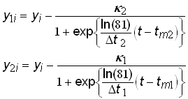
(14)
where y1i and y2i are the component growth variables, which are plotted in the inset of figure 2.
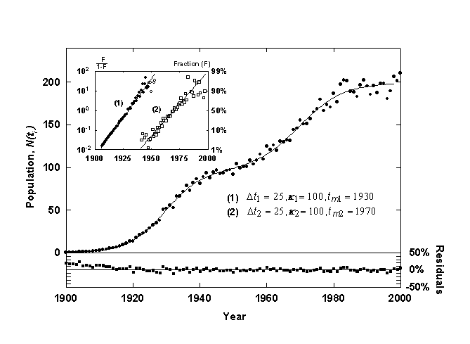
Figure 3. Example of a Bi-Logistic growth curve generated with 3% relative Gaussian error. The inset shows the component growth curves linearized with the Fisher-Pry transform. The lower panel shows the residuals from the fit in percent deviation from the fitted curve.
The two data sets (ti, y1i) and (ti, y2i), can also be plotted as a linear function of time by utilizing the Fisher-Pry transform, as shown in the inset of Figure 3, with the circles designating (ti, y1i) and the squares designating (ti, y2i). When the second logistic pulse is below 1% of saturation (k2), the first component data set (ti, y1i>) is essentially identical to the raw data, (ti, yi), and it is plotted with solid circles. After this, the data are plotted with open circles to indicate that the data have been transformed. The second component growth data set (ti, y2i) is plotted with hollow squares to indicated that these data have also been transformed. The linear form of the Bi-logistic facilitates morphological analysis and comparison to other Bi-logistic processes.
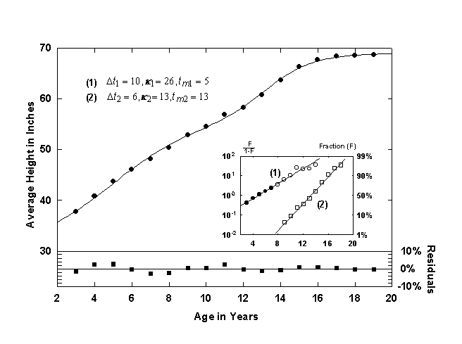
Figure 4. Average height of American Boys with a Bi-Logistic growth curve. Note that the Bi-logistic curve is offset by 30 inches in order to account for early growth (ages 0 to 3). Source of data: [12].
A well-known growth process involving two growth spurts is shown in Figure 4, the average height of boys ages 3 to 19, in this case, American [12]. Two S-shaped growth pulses are clearly visible. The first growth pulse shown is centered at 5 years and has a characteristic growth time, Dt, of 10 years. The second growth pulse, called the “prepubertal acceleration” or the “adolescent spurt” is shorter and is centered at 13 years old. This growth pulse saturates at 68.7 inches, the average height of American men. The inset shows the Fisher-Pry linear transform of the two growth pulses.
The residuals are useful in determining how well the Bi-logistic model fits the data. If a system is well modeled by the Bi-logistic function, then the residuals will contain only noise, and the residuals will be randomly distributed around zero. The residuals can also tell a lot about the error structure. The lower part of Figures 3 and 4 show the residuals of the fit on the two time-series data. The residuals are shown as the percent deviation from the estimated value
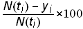
residuals in percent deviation =.(15)
Many time series data sets from systems that are studied with logistics contain error that is relative to the growth level, which can change by orders of magnitude in the duration of the process. Accordingly, it is useful to analyze the residuals in percent deviation. While the ordinary least-squares technique used for analysis assumes constant error variance, it might be advantageous to use a regression method that assumes constant relative error, thus weighing the early growth data more heavily than the later data. However, early growth data are often unreliable, as processes may also not be well recorded or established. Thus there is a trade off between assuming relative error and constant error. The effect can be seen in the comparatively high levels of error present in the early data on the residual plot of the generated time-series data (figure 3), which was fit assuming constant error. More research is needed to determine the error structure of historical data-sets and on regression techniques that yield the best parameter estimates. Monte-Carlo techniques could be used to generate sample data sets with different error structures, and the subsequent analysis would be useful in determining confidence intervals for the Bi-logistic model parameters. Residual analysis could also identify “slices” of data that are especially noise-free and might be more heavily weighted when fitting.
Taxonomy of the Bi-logistic
A continuous spectrum of curves can be generated from the Bi-logistic model. However, it is useful to distinguish four basic patterns of Bi-logistic growth in order to develop a taxonomy of curves that can be used as a reference when analyzing systems where the shapes of the two underlying logistic trends are not already known. As mentioned, the regression routine used requires initial estimates, and a taxonomy is useful in this regard.
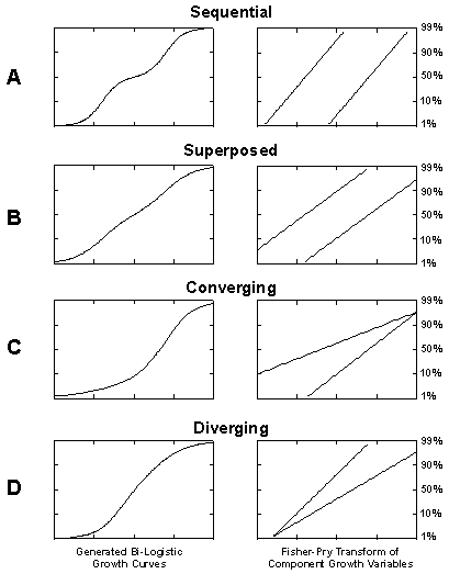
Figure 5. Taxonomy of the Bi-logistic growth model.
Figure 5 shows four hypothetical curves and their linearized versions.
Curve A of Figure 5 shows a Bi-logistic curve with two almost non-overlapping logistic growth pulses, dubbed the “sequential logistic”. The second pulse does not start growing until the first pulse has reached about 99% of saturation k1. This shape Bi-logistic characterizes a system which pauses between growth phases.
The B curve shows a Bi-logistic where the second pulse starts growing when the first pulse has reached about 50% of saturation. This “superposed” Bi-logistic growth model characterizes systems that contain two processes of a similar nature growing concurrently except for a displacement in the midpoints of the curves.
Curve C shows a growth process where a first pulse of logistic growth is joined by a second faster pulse, dubbed the “converging” logistic model, as the two pulses culminate about the same time. Often an advance in technology will allow both the carrying capacity and the growth rate of a system to increase, causing the second pulse to rise from the first with both a faster characteristic Dt, and higher carrying capacity,k.
Curve D shows a “diverging” Bi-logistic curve where two logistic growth processes begin at the same time but grow with different rates and carrying capacities defined from the start. It is noteworthy that curves C and D are S-shaped but asymmetric. They do not “look logistic.”
Examples and Results
A wide variety of historical time-series data sets were analyzed with the Bi-logistic model. The data sets exhibited here show the four types of Bi-logistic growth described above. The data sets chosen all show growth processes that have neared saturation in order to permit analysis of the residuals for the entire growth process. The data sets were also fitted with a single logistic growth pulse to check the improvement in fit by the Bi-logistic.
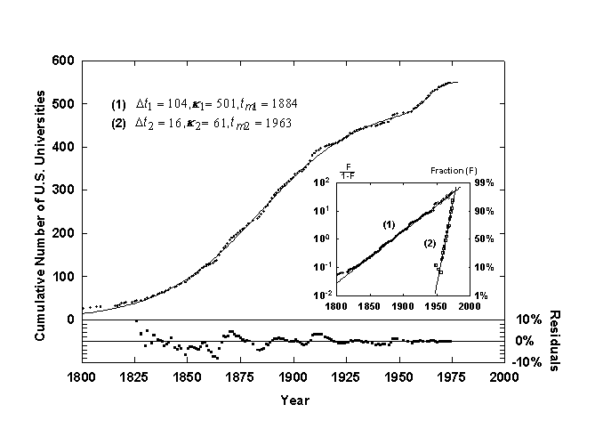
Figure 6. Growth of U.S. universities with a Bi-Logistic growth curve. Source of data: [13].
A sequential Bi-logistic is shown in figure 6, the growth of U.S. universities since 1700, as tabulated from the founding dates provided in Webster’s New Collegiate Dictionary [13]. The first pulse saturates at a k of 500 universities with the point of inflection and fastest rate of growth, tm, occurring in 1885. This is when many states inaugurated their public university systems. The second, smaller logistic pulse starts in 1950 when the first pulse has reached about 95% of saturation and has a much quicker characteristic growth time, Dt, of about 15 years. This pulse represents largely the creation of additional daughter campuses of state universities, a smaller niche to fill than the founding of universities for the U.S. as a whole.
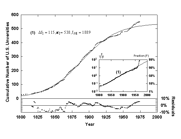
Figure 7. Growth of U.S. universities with a single logistic growth curve. Source of data: [13].
To indicate the superiority of the Bi-logistic, consider Figure 7, which shows the same university data fitted with a single logistic curve. Optical inspection of the fitted curve as well as analysis of the residuals show that the Bi-logistic model fits the data much better than a single logistic curve. The residuals of the early data (1600-1800) have small absolute error but because the growth level is low the percent error is very high (~100%). As mentioned, this deviation is caused in part by the non-weighted regression algorithm used. The early growth of systems (below 10% of final saturation) is also suspect because feedback mechanisms that are assumed for logistic growth might not be in place yet, and thus the growth is probably not firmly logistic until a growth level of about 10% of the final saturation value has been reached.
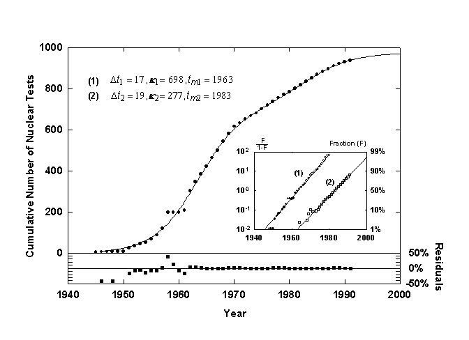
Figure 8. U.S. nuclear weapons tests with a Bi-logistic growth curve. Source of data: [14].
Figure 8 shows the cumulative number of U.S. nuclear weapons tests [14] with a superposed Bi-logistic curve. The Bi-logistic provides an excellent fit, as shown by the residuals. The fastest rate of growth of the first pulse occurred in 1963, following the Cuban missile crisis. While the first logistic pulse was largely the race to develop bombs with higher yields, the second pulse, centered in 1983 and nearing saturation now, is probably due to research on reliability and specific weapons designed for tactical use. The Bi-logistic model predicts that we are at 90% of saturation of the latest pulse. Processes often expire around 90%, though sometimes processes overshoot. The residuals show the extraordinary, deviant increase in U.S. tests after the scare of the 1957 sputnik launch.
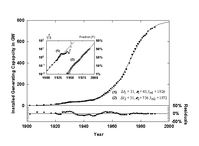
Figure 9. U.S. installed electric generating capacity with a Bi-logistic growth curve. Source of data: [15, 16].
Figure 9 shows the U.S. installed electric generating capacity [15,16] with a converging Bi-logistic curve. The first logistic pulse saturates at about 43 GW and is centered in 1926. A second shorter but much higher pulse begins in about 1940 and is at about 90% of saturation now. Ausubel and Marchetti [17] provide a detailed analysis of the underlying mechanisms affecting the electrification of the U.S. The first pulse of growth is associated with pure substitution, for example, the replacement of water mills and gaslight by more efficient and convenient electric devices. The second and much larger growth pulse is due to the increase in demand of electricity for energy functions that could not be easily fulfilled before electrification, ranging from TV’s to space cooling. The pair of pulses have more or less saturated now. A third electric pulse might be starting with the rapid increase in demand for information handling and new concepts in electric transport.
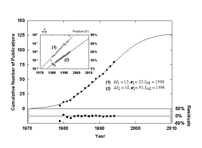
Figure 10. Cumulative number of published works, Jesse H. Ausubel, with a Bi-logistic growth curve. Source of data: personal communication.
Figure 10 shows the cumulative number of publications written or edited by my colleague, Jesse H. Ausubel, fitted with a diverging Bi-logistic curve. The first smaller, steeper pulse consists of committee reports and other collective documents associated with his work as a staff officer and study director. The second longer and higher pulse consists of research papers of which Ausubel is an author. His dual professional career is made neatly apparent by the Bi-logistic.
Issues and Conclusion
To analyze time series data sets where the simple logistic curve provides a poor fit, many other growth models have been examined [18] , such as the Gompertz function. These data sets might contain multiple growth pulses that would be better modeled by the Bi-logistic. Some of the other models introduce higher-order parameters where the physical interpretation is less clear than in the case of the Bi-logistic. More research is needed in order to determine if the Bi-logistic model performs as well as more complex non-symmetrical growth functions. Complex systems can also undergo or consist of more than two pulses of growth, and research is needed into the feasibility of extending the Bi-logistic model into an arbitrary sum of simple logistics. Of course, with enough parameters anything can be fit.
The logistic growth function has proven useful in modeling a wide variety of phenomena in the growth of systems. However, complex systems rarely follow a single S-shaped trajectory. The Bi-logistic function is effective in modeling systems that contain two logistic growth pulses. The Bi-logistic is attractive because it is a parsimonious model to which we can still attach clear physical interpretations.
Acknowledgments: I am grateful to Jesse Ausubel, John Helm, Robert Herman, Arnulf Grübler, Cesare Marchetti, Nebojsa Nakicenovic, and Andy Solow for advice and assistance.
References
- Kingsland, S., The Refractory Model: The Logistic Curve and the History of Population Ecology, The Quarterly Review of Biology 57, 29-52 (1982).
- Marchetti, C., Branching out into the Universe, in Diffusion of Technologies and Social Behavior, N. Nakicenovic and A. Grübler, eds., Springer-Verlag, New York, NY, 1991.
- Grübler, A., The Rise and Fall of Infrastructures, Springer-Verlag, New York, NY, 1990.
- Oliver, R. M., Saturation Models: A Brief Survey and Critique, Journal of Forecasting (Special Issue on Predicting Saturation and Logistic Growth) 7, 15-255 (1988).
- Young, P., Technological Growth Curves: A Competition of Forecasting Models, Technological Forecasting and Social Change 44, 375-389 (1993).
- Stone, R., Sigmoids, Bulletin in Applied Statistics 7, 59-119 (1980).
- Nakicenovic, N., U.S. Transport Infrastructures, in Cities and Their Vital Systems, J. Ausubel and R. Herman, eds., National Academy Press, Washington, D.C., 1988.
- Reed, H.S. and Holland, R. H., The Growth of an Annual Plant Helianthus, Proceedings of the National Academy of Sciences (USA), 5, 135-144 (1919).
- Fisher, J.C., and Pry, R. H., A Simple Substitution Model of Technological Change, Technological Forecasting and Social Change 3, 75-88 (1971).
- Montroll, E. W., Social Dynamics and the Quantifying of Social Forces, Proceedings of the National Academy of Sciences (USA) 75(10), 4633-37 (1978).
- Press, W. H., Teukolsky, S. A., Vetterling, W. T., and Flannery, B. P., Numerical Recipes in C: The Art of Scientific Computing 2nd ed., Cambridge University Press, New York, NY, 1992.
- Krogman, W. M., Child Growth, University of Michigan Press, Ann Arbor, MI, 1972.
- Woolf, H. B., ed., Webster’s New Collegiate Dictionary, Merriam-Webster, Springfield, MA, 1979.
- Stockholm International Peace Research Institute Yearbook 1992, Oxford University Press, New York, 1992.
- U.S. Bureau of the Census, Historical Statistics of the United States, Washington, D.C., 1975.
- U.S. Bureau of the Census, Statistical Abstract of the United States, Washington, D.C., (Various Years).
- Ausubel, J. and Marchetti, C., Elektron, Forthcoming in Technological Trajectories and the Human Environment, J. Ausubel and D. Langford, eds., National Academy Press, Washington, D.C.
- Posch, M., Grübler, A., and Nakicenovic, N., Methods of Estimating S-Shaped Growth Functions, International Institute for Applied Systems Analysis, Laxenburg, Austria, 1987.
Microphysics and Macrohistory
Carrying Capacity: A Model with Logistically Varying Limits
If you are unable to view these formats, email us at phe@rockefeller.edu for a reprint.
These papers were prepared using Donald Knuth’s open-source TeX typesetting environment, with the AMS-LaTeX macro package, and the dvips and pdftex programs to create Postscript and PDF versions. All these tools are available in the excellent teTeX-1.0 distribution, available at https://www.tug.org/tetex/. You can find more information on TeX at the TeX users group, https://www.tug.org.
Death and the Human Environment: The United States in the 20th Century
AN INTRODUCTION TO DEADLY COMPETITION
Our subject is the history of death. Researchers have analyzed the time dynamics of numerous populations-nations, companies, products, technologies–competing to fill a niche or provide a given service. Here we review killers, causes of death, as competitors for human bodies. We undertake the analysis to understand better the role of the environment in the evolution of patterns of mortality. Some of the story will prove familiar to public health experts. The story begins in the environment of water, soil, and air, but it leads elsewhere.
Our method is to apply two models developed in ecology to study growth and decline of interacting populations. These models, built around the logistic equation, offer a compact way of organizing numerous data and also enable prediction. The first model represents simple S-shaped growth or decline.[1] The second model represents multiple, overlapping and interacting processes growing or declining in S-shaped paths.[2] Marchetti first suggested the application of logistic models to causes of death in 1982.[3]
The first, simple logistic model assumes that a population grows exponentially until an upper limit inherent in the system is approached, at which point the growth rate slows and the population eventually saturates, producing a characteristic S-shaped curve. A classic example is the rapid climb and then plateau of the number of people infected in an epidemic. Conversely, a population such as the uninfected sleds downward in a similar logistic curve. Three variables characterize the logistic model: the duration of the process (Dt), defined as the time required for the population to grow from 10 percent to 90 percent of its extent; the midpoint of the growth process, which fixes it in time and marks the peak rate of change; and the saturation or limiting size of the population. For each of the causes of death that we examine, we analyze this S-shaped “market penetration” (or withdrawal) and quantify the variables.
Biostatisticians have long recognized competing risks, and so our second model represents multi-species competition. Here causes of death compete with and, if fitter in an inclusively Darwinian sense, substitute for one another. Each cause grows, saturates, and declines, and in the process reduces or creates space for other causes within the overall niche. The growth and decline phases follow the S-shaped paths of the logistic law.
The domain of our analysis is the United States in the 20th century. We start systematically in the year 1900, because that is when reasonably reliable and complete U.S. time series on causes of death begin. Additionally, 1900 is a commencement because the relative importance of causes of death was rapidly and systematically changing. In earlier periods causes of death may have been in rough equilibrium, fluctuating but not systematically changing. In such periods, the logistic model would not apply. The National Center for Health Statistics and its predecessors collect the data analyzed, which are also published in volumes issued by the U.S. Bureau of the Census.[4]
The data present several problems. One is that the categories of causes of death are old, and some are crude. The categories bear some uncertainty. Alternative categories and clusters, such as genetic illnesses, might be defined for which data could be assembled. Areas of incomplete data, such as neonatal mortality, and omissions, such as fetal deaths, could be addressed. To complicate the analysis, some categories have been changed by the U.S. government statisticians since 1900, incorporating, for example, better knowledge of forms of cancer.
Other problems are that the causes of death may be unrecorded or recorded incorrectly. For a decreasing fraction of causes of death, no “modern” cause is assigned. We assume that the unassigned or “other” deaths, which were numerous until about 1930, do not bias the analysis of the remainder. That is, they would roughly pro-rate to the assigned causes. Similarly, we assume no systematic error in early records.
Furthermore, causes are sometimes multiple, though the death certificate requires that ultimately one basic cause be listed.[5] This rule may hide environmental causes. For example, infectious and parasitic diseases thrive in populations suffering drought and malnutrition. The selection rule dictates that only the infectious or parasitic disease be listed as the basic cause. For some communities or populations the bias could be significant, though not, we believe, for our macroscopic look at the 20th century United States.
The analysis treats all Americans as one population. Additional analyses could be carried out for subpopulations of various kinds and by age group.[6] Comparable analyses could be prepared for populations elsewhere in the world at various levels of economic development.[7]
With these cautions, history still emerges.
As a reference point, first observe the top 15 causes of death in America in 1900 (Table 1). These accounted for about 70 percent of the registered deaths. The remainder would include both a sprinkling of many other causes and some deaths that should have been assigned to the leading causes. Although heart disease already is the largest single cause of death in 1900, the infectious diseases dominate the standings.
Death took 1.3 million in the United States in 1900. In 1997 about 2.3 million succumbed. While the population of Americans more than tripled, deaths in America increased only 1.7 times because the death rate halved (Figure 1). As we shall see, early in the century the hunter microbes had better success.
Table 1. U.S. death rate per 100,000 population for leading causes, 1900. For source of data, see Note 4.
| Cause | Rate | Mode of Transmission | |
| 1. | Major Cardiovascular Disease | 345 | [N.A.] |
| 2. | Influenza, Pneumonia | 202 | Inhalation,Intimate Contact |
| 3. | Tuberculosis | 194 | Inhalation,Intimate Contact |
| 4. | Gastritis, Colitus,Enteritis, and Duodenitis | 142 | Contaminated Waterand Food |
| 5. | All Accidents | 72 | [Behavioral] |
| 6. | Malignant Neoplasms | 64 | [N.A.] |
| 7. | Diphtheria | 40 | Inhalation |
| 8. | Typhoid and ParatyphoidFever | 31 | Contaminated Water |
| 9. | Measles | 13 | Inhalation, Intimate Contact |
| 10. | Cirrhosis | 12 | [Behavioral] |
| 11. | Whooping Cough | 12 | Inhalation, Intimate Contact |
| 12. | Syphilis and Its Sequelae | 12 | Sexual Contact |
| 13. | Diabetes Mellitus | 11 | [N.A.] |
| 14. | Suicide | 10 | [Behavioral] |
| 15. | Scarlet Fever and Streptococcal Sore Throat | 9 | Inhalation, Intimate Contact |
DOSSIERS OF EIGHT KILLERS
Let us now review the histories of eight causes of death: typhoid, diphtheria, the gastrointestinal family, tuberculosis, pneumonia plus influenza, cardiovascular, cancer, and AIDS.
For each of these, we will see first how it competes against the sum of all other causes of death. In each figure we show the raw data, that is, the fraction of total deaths attributable to the killer, with a logistic curve fitted to the data. In an inset, we show the identical data in a transform that renders the S-shaped logistic curve linear.[8] It also normalizes the process of growth or decline to one (or to 100 percent). Thus, in the linear transform the fraction of deaths each cause garners, which is plotted on a semi-logarithmic scale, becomes the percent of its own peak level (taken as one hundred percent). The linear transform eases the comparison among cases and the identification of the duration and midpoint of the processes, but also compresses fluctuations.
Typhoid (Figure 2) is a systemic bacterial infection caused primarily by Salmonella typhi.[9] Mary Mallon, the cook (and asymptomatic carrier) popularly known as Typhoid Mary, was a major factor in empowering the New York City Department of Health at the turn of the century. Typhoid was still a significant killer in 1900, though spotty records show it peaked in the 1870s. In the 1890s, Walter Reed, William T. Sedgewick, and others determined the etiology of typhoid fever and confirmed its relation to sewage-polluted water. It took about 40 years to protect against typhoid, with 1914 the year of inflection or peak rate of decline.
Diphtheria (Figure 2) is an acute infectious disease caused by diphtheria toxin of the Corynebacterium diphtheriae. In Massachusetts, where the records extend back further than for the United States as a whole, diphtheria flared to 196 per 100,000 in 1876, or about 10 percent of all deaths. Like typhoid, diphtheria took 40 years to defense, centered in 1911. By the time the diphtheria vaccine was introduced in the early 1930s, 90 percent of its murderous career transition was complete.
Next comes the category of diseases of the gut (Figure 2). Deaths here are mostly attributed to acute dehydrating diarrhea, especially in children, but also to other bacterial infections such as botulism and various kinds of food poisoning. The most notorious culprit was the Vibrio cholerae. In 1833, while essayist Ralph Waldo Emerson was working on his book Nature, expounding the basic benevolence of the universe, a cholera pandemic killed 5 to 15 percent of the population in many American localities where the normal annual death rate from all causes was 2 or 3 percent.
In 1854 in London a physician and health investigator, John Snow, seized the idea of plotting the locations of cholera deaths on a map of the city. Most deaths occurred in St. James Parish, clustered about the Broad Street water pump. Snow discovered that cholera victims who lived outside the Parish also drew water from the pump. Although consumption of the infected water had already peaked, Snow’s famous removal of the pump handle properly fixed in the public mind the means of cholera transmission.[10] In the United States, the collapse of cholera and its relations took about 60 years, centered on 1913. As with typhoid and diphtheria, sanitary engineering and public health measures addressed most of the problem before modern medicine intervened with antibiotics in the 1940s.
In the late 1960s, deaths from gastrointestinal disease again fell sharply. The fall may indicate the widespread adoption of intravenous and oral rehydration therapies and perhaps new antibiotics. It may also reflect a change in record-keeping.
Tuberculosis (Figure 2) refers largely to the infectious disease of the lungs caused by Mycobacterium tuberculosis. In the 1860s and 1870s in Massachusetts, TB peaked at 375 deaths per 100,000, or about 15 percent of all deaths. Henry David Thoreau, author of Walden: or, Life in the Woods, died of bronchitis and tuberculosis at the age of 45 in 1862. TB took about 53 years to jail, centered in 1931. Again, the pharmacopoeia entered the battle rather late. The multi-drug therapies became effective only in the 1950s.
Pneumonia and influenza are combined in Figure 3. They may comprise the least satisfactory category, mixing viral and bacterial aggressors. Figure 3 includes Influenza A, the frequently mutating RNA virus believed to have induced the Great Pandemic of 1918-1919 following World War I, when flu seized about a third of all corpses in the United States. Pneumonia and influenza were on the loose until the 1930s. Then, in 17 years centered on 1940 the lethality of pneumonia and influenza tumbled to a plateau where “flu” has remained irrepressibly for a half century.
Now we shift from pathogens to a couple of other major killers. Major cardiovascular diseases, including heart disease, hypertension, cerebrovascular diseases, atherosclerosis, and associated renal diseases display their triumphal climb and incipient decline in Figure 3. In 1960, about 55 percent of all fatal attacks were against the heart and its allies, culminating a 60-year climb. Having lost 14 points of market share in the past 40 years, cardiovascular disease looks vulnerable. Other paths descend quickly, once they bend downward. We predict an 80-year drop to about 20 percent of American dead. Cardiovascular disease is ripe for treatment through behavioral change and medicine.
A century of unremitting gains for malignant neoplasms appears neatly in Figure 3. According to Ames et al., the culprits are ultimately the DNA-damaging oxidants.[11] One might argue caution in lumping together lung, stomach, breast, prostate, and other cancers. Lung and the other cancers associated with smoking account for much of the rising slope. However, the cancers whose occurrence has remained constant are also winning share if other causes of death diminish. In the 1990s the death rate from malignancies flattened, but the few years do not yet suffice to make a trend. According to the model, cancer’s rise should last 160 years and at peak account for 40 percent of American deaths.
The spoils of AIDS, a meteoric viral entrant, are charted in Figure 3. The span of data for AIDS is short, and the data plotted here may not be reliable. Pneumonia and other causes of death may mask AIDS’ toll. Still, this analysis suggests AIDS reached its peak market of about 2 percent of deaths in the year 1995. Uniquely, the AIDS trajectory suggests medicine sharply blocked a deadly career, stopping it about 60% of the way toward its project fulfillment.
Now look at the eight causes of death as if it were open hunting season for all (Figure 4). Shares of the hunt changed dramatically, and fewer hunters can still shoot to kill with regularity. We can speculate why.
BY WATER, BY AIR
First, consider what we label the aquatic kills: a combination of typhoid and the gastrointestinal family. They cohere visually and phase down by a factor of ten over 33 years centered on 1919 (Figure 5).
Until well into the 19th century, towndwellers drew their water from local ponds, streams, cisterns, and wells.[12] They disposed of the wastewater from cleaning, cooking, and washing by throwing it on the ground, into a gutter, or a cesspool lined with broken stones. Human wastes went to privy vaults, shallow holes lined with brick or stone, close to home, sometimes in the cellar. In 1829 residents of New York City deposited about 100 tons of excrement each day in the city soil. Scavengers collected the “night soil” in carts and dumped it nearby, often in streams and rivers.
Between 1850 and 1900 the share of the American population living in towns grew from about 15 to about 40 percent. The number of cities over 50,000 grew from 10 to more than 50. Increasing urban density made waste collection systems less adequate. Overflowing privies and cesspools filled alleys and yards with stagnant water and fecal wastes. The growing availability of piped-in water created further stress. More water was needed for fighting fires, for new industries that required pure and constant water supply, and for flushing streets. To the extent they existed, underground sewers were designed more for storm water than wastes. One could not design a more supportive environment for typhoid, cholera, and other water-borne killers.
By 1900 towns were building systems to treat their water and sewage. Financing and constructing the needed infrastructure took several decades. By 1940 the combination of water filtration, chlorination, and sewage treatment stopped most of the aquatic killers.
Refrigeration in homes, shops, trucks, and railroad boxcars took care of much of the rest. The chlorofluorocarbons (CFCs) condemned today for thinning the ozone layer were introduced in the early 1930s as a safer and more effective substitute for ammonia in refrigerators. The ammonia devices tended to explode. If thousands of Americans still died of gastrointestinal diseases or were blown away by ammonia, we might hesitate to ban CFCs.
Let us move now from the water to the air (Figure 6). “Aerial” groups all deaths from influenza and pneumonia, TB, diphtheria, measles, whooping cough, and scarlet fever and other streptococcal diseases. Broadly speaking these travel by air. To a considerable extent they are diseases of crowding and unfavorable living and working conditions.
Collectively, the aerial diseases were about three times as deadly to Americans as their aquatic brethren in 1900. Their breakdown began more than a decade later and required almost 40 years.
The decline could be decomposed into several sources. Certainly large credit goes to improvements in the built environment: replacement of tenements and sweatshops with more spacious and better ventilated homes and workplaces. Huddled masses breathed free. Much credit goes to electricity and cleaner energy systems at the level of the end user.
Reduced exposure to infection may be an unrecognized benefit of shifting from mass transit to personal vehicles. Credit obviously is also due to nutrition, public health measures, and medical treatments.
The aerial killers have kept their market share stable since the mid-1950s. Their persistence associates with poverty; crowded environments such as schoolrooms and prisons; and the intractability of viral diseases. Mass defense is more difficult. Even the poorest Bostonians or Angelenos receive safe drinking water; for the air, there is no equivalent to chlorination.
Many aerial attacks occurred in winter, when indoor crowding is greatest. Many aquatic kills were during summer, when the organic fermenters were speediest. Diarrhea was called the summer complaint. In Chicago between 1867 and 1925 a phase shift occurred in the peak incidence of mortality from the summer to the winter months.[13] In America and other temperate zone industrialized countries, the annual mortality curve has flattened during this century as the human environment has come under control. In these countries, most of the faces of death are no longer seasonal.
BY WAR, BY CHANCE?
Let us address briefly the question of where war and accidents fit. In our context we care about war because disputed control of natural resources such as oil and water can cause war. Furthermore, war leaves a legacy of degraded environment and poverty where pathogens find prey. We saw the extraordinary spike of the flu pandemic of 1918-1919.
War functions as a short-lived and sometimes intense epidemic. In this century, the most intense war in the developed countries may have been in France between 1914-1918, when about one-quarter of all deaths were associated with arms.[14] The peak of 20th century war deaths in the United States occurred between 1941-1945 when about 7 percent of all deaths were in military service, slightly exceeding pneumonia and influenza in those years.
Accidents, which include traffic, falls, drowning, and fire follow a dual logic. Observe the shares of auto and all other accidents in the total kills in the United States during this century (Figure 7). Like most diseases, fatal non-auto accidents have dropped, in this case rather linearly from about 6 percent to about 2 percent of all fatalities. Smiths and miners faced more dangers than office workers. The fall also reflects lessening loss of life from environmental hazards such as floods, storms, and heat waves.
Auto accidents do not appear accidental at all but under perfect social control. On the roads, we appear to tolerate a certain range of risk and regulate accordingly, an example of so-called risk homeostasis.[15] The share of killing by auto has fluctuated around 2 percent since about 1930, carefully maintained by numerous changes in vehicles, traffic management, driving habits, driver education, and penalties.
DEADLY ORDER
Let us return to the main story. Infectious diseases scourged the 19th century. In Massachusetts in 1872, one of the worst plague years, five infectious diseases, tuberculosis, diphtheria, typhoid, measles, and smallpox, alone accounted for 27 percent of all deaths. Infectious diseases thrived in the environment of the industrial revolution’s new towns and cities, which grew without modern sanitation.
Infectious diseases, of course, are not peculiarly diseases of industrialization. In England during the intermittent plagues between 1348-1374 half or more of all mortality may have been attributable to the Black Death.[16] The invasion of smallpox into Central Mexico at the time of the Spanish conquest depopulated central Mexico.[17] Gonorrhea depopulated the Pacific island of Yap.[18]
At the time of its founding in 1901, our institution, the Rockefeller Institute for Medical Research as it was then called, appropriately focused on the infectious diseases. Prosperity, improvements in environmental quality, and science diminished the fatal power of the infectious diseases by an order of magnitude in the United States in the first three to four decades of this century. Modern medicine has kept the lid on.[19]
If infections were the killers of reckless 19th century urbanization, cardiovascular diseases were the killers of 20th century modernization. While avoiding the subway in your auto may have reduced the chance of influenza, it increased the risk of heart disease. Traditionally populations fatten when they change to a “modern” lifestyle. When Samoans migrate to Hawaii and San Francisco or live a relatively affluent life in American Samoa, they gain between 10 and 30 kg.[20]
The environment of cardiovascular death is not the Broad Street pump but offices, restaurants, and cars. So, heart disease and stroke appropriately roared to the lead in the 1920s.
Since the 1950s, however, cardiovascular disease has steadily lost ground to a more indefatigable terminator, cancer. In our calculation, cancer passed infection for the #2 spot in 1945. Americans appear to have felt the change. In that year Alfred P. Sloan and Charles Kettering channeled some of the fortune they had amassed in building the General Motors Corporation to found the Sloan-Kettering Cancer Research Center.
Though cancer trailed cardiovascular in 1997 by 41 to 23 percent, cancer should take over as the nation’s #1 killer by 2015, if long-run dynamics continue as usual (Figure 8). The main reasons are not environmental. Doll and Peto estimate that only about 5 percent of U.S. cancer deaths are attributable to environmental pollution and geophysical factors such as background radiation and sunlight.[21]
The major proximate causes of current forms of cancer, particularly tobacco smoke and dietary imbalances, can be reduced. But if Ames and others are right that cancer is a degenerative disease of aging, no miracle drugs should be expected, and one form of cancer will succeed another, assuring it a long stay at the top of the most wanted list. In the competition among the three major families of death, cardiovascular will have held first place for almost 100 years, from 1920 to 2015.
Will a new competitor enter the hunt? As various voices have warned, the most likely suspect is an old one, infectious disease.[22] Growth of antibiotic resistance may signal re-emergence. Also, humanity may be creating new environments, for example, in hospitals, where infection will again flourish. Massive population fluxes over great distances test immune systems with new exposures. Human immune systems may themselves weaken, as children grow in sterile apartments rather than barnyards.[23] Probably most important, a very large number of elderly offer weak defense against infections, as age-adjusted studies could confirm and quantify. So, we tentatively but logically and consistently project a second wave of infectious disease. In Figure 9 we aggregate all major infectious killers, both bacterial and viral. The category thus includes not only the aquatics and aerials discussed earlier, but also septicemia, syphilis, and AIDS.[24] A grand and orderly succession emerges.
SUMMARY
Historical examination of causes of death shows that lethality may evolve in consistent and predictable ways as the human environment comes under control. In the United States during the 20th century infections became less deadly, while heart disease grew dominant, followed by cancer. Logistic models of growth and multi-species competition in which the causes of death are the competitors describe precisely the evolutionary success of the killers, as seen in the dossiers of typhoid, diphtheria, the gastrointestinal family, pneumonia/influenza, cardiovascular disease, and cancer. Improvements in water supply and other aspects of the environment provided the cardinal defenses against infection. Environmental strategies appear less powerful for deferring the likely future causes of death. Cancer will overtake heart disease as the leading U.S. killer around the year 2015 and infections will gradually regain their fatal edge. If the orderly history of death continues.
FIGURES
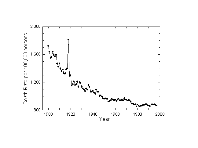
Figure 1. Crude Death Rate: U.S. 1900-1997. Sources of data: Note 4.
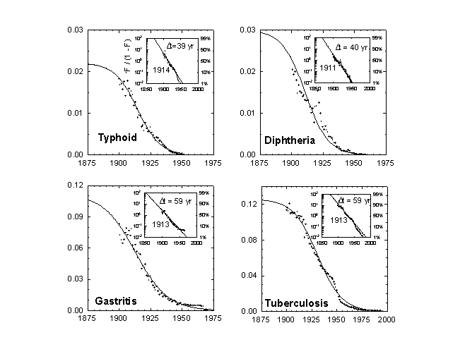
Figure 2a. Typhoid and Paratyphoid Fever as a Fraction of All Deaths: U.S. 1900-1952. The larger panel shows the raw data and a logistic curve fitted to the data. The inset panel shows the same data and a transform that renders the S-shaped curve linear and normalizes the process to 1. “F” refers to the fraction of the process completed. Here the time it takes the process to go from 10 percent to 90 percent of its extent is 39 years, and the midpoint is the year 1914. Source of data: Note 4.
Figure 2b. Diphtheria as a Fraction of All Deaths: U.S. 1900-1956. Source of data: Note 4.
Figure 2c. Gastritis, Duodenitis, Enteritis, and Colitis as a Fraction of All Deaths: U.S. 1900-1970. Source of data: Note 4.
Figure 2d. Tuberculosis, All Forms, as a Fraction of All Deaths: U.S. 1900-1997. Sources of data: Note 4.
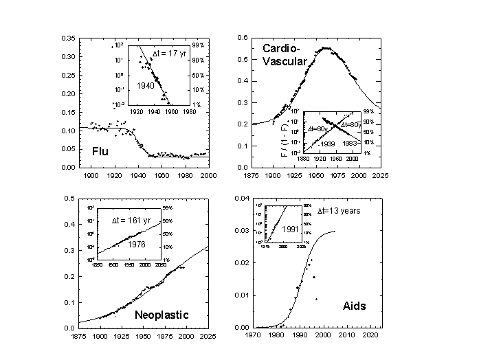
Figure 3a. Pneumonia and Influenza as a Fraction of All Deaths: U.S. 1900-1997. Note the extraordinary pandemic of 1918-1919. Sources of data: Note 4.
Figure 3b. Major Cardiovascular Diseases as a Fraction of All Deaths: U.S. 1900-1997. In the inset, the curve is decomposed into upward and downward logistics which sum to the actual data values. The midpoint of the 60-year rise of cardiovascular disease was the year 1939, while the year 1983 marked the midpoint of its 80-year decline. Sources of data: Note 4.
Figure 3c. Malignant Neoplasms as a Fraction of All Deaths: U.S. 1900-1997. Sources of data: Note 4.
Figure 3d. AIDS as a Fraction of All Deaths: U.S. 1981-1997. Sources of data: Note 4.
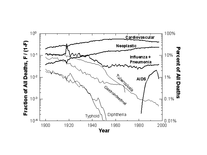
Figure 4. Comparative Trajectories of Eight Killers: U.S. 1900-1997. The scale is logarithmic, with fraction of all deaths shown on the left scale with the equivalent percentages marked on the right scale. Sources of data: Note 4.
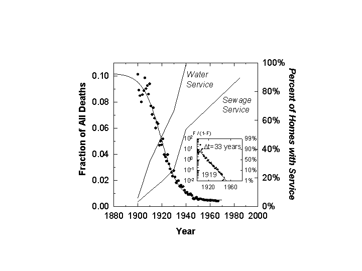
Figure 5. Deaths from Aquatically Transmitted Diseases as a Fraction of All Deaths: U.S. 1900-1967. Superimposed is the percentage of homes with water and sewage service (right scale). Source of data: Note 4.
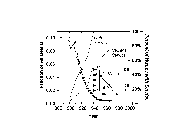
Figure 6. Deaths from Aerially Transmitted Diseases as a Fraction of All Deaths: U.S. 1900-1997. Sources of data: Note 4.
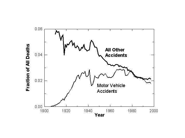
Figure 7. Motor Vehicle and All Other Accidents as a Fraction of All Deaths: U.S. 1900-1997. Sources of data: Note 4.
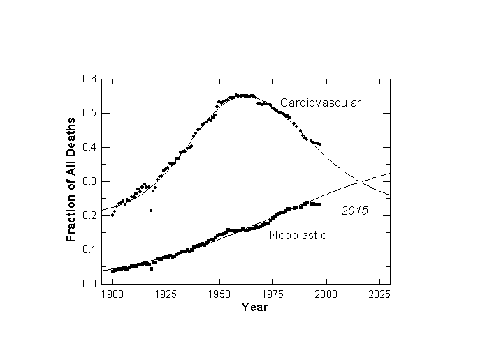
Figure 8. Major Cardiovascular Diseases and Malignant Neoplasms as a Fraction of All U.S. Deaths: 1900-1997. The logistic model predicts (dashed lines) Neoplastic will overtake Cardiovascular as the number one killer in 2015. Sources of data: Note 4.
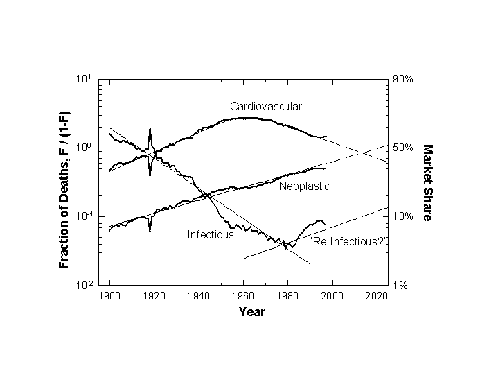
Figure 9. Major Causes of Death Analyzed with a Multi-species Model of Logistic Competition. The fractional shares are plotted on a logarithmic scale which makes linear the S-shaped rise and fall of market shares.
Notes
[1] On the basic model see: Kingsland SE. Modeling Nature: Episodes in the History of Population Ecology. Chicago: University of Chicago Press, 1985. Meyer PS. Bi-logistic growth. Technological Forecasting and Social Change 1994;47:89-102.
[2] On the model of multi-species competition see Meyer PS, Yung JW, Ausubel JH. A Primer on logistic growth and substitution: the mathematics of the Loglet Lab software. Technological Forecasting and Social Change 1999;61(3):247-271.
[3] Marchetti C. Killer stories: a system exploration in mortal disease. PP-82-007. Laxenburg, Austria: International Institute for Applied Systems Analysis, 1982. For a general review of applications see: Nakicenovic N, Gruebler A, eds. Diffusion of Technologies and Social Behavior. New York: Springer-Verlag, 1991.
[4] U.S. Bureau of the Census, Historical Statistics of the United States: Colonial Times to 1970, Bicentennial Editions, Parts 1 & 2. Washington DC: U.S. Bureau of the Census: 1975. U.S. Bureau of the Census, Statistical Abstract of the United States: 1999 (119th edition). Washington DC: 1999, and earlier editions in this annual series.
[5] Deaths worldwide are assigned a “basic cause” through the use of the “Rules for the Selection of Basic Cause” stated in the Ninth Revision of the International Classification of Diseases. Geneva: World Health Organization. These selection rules are applied when more than one cause of death appears on the death certificate, a fairly common occurrence. From an environmental perspective, the rules are significantly biased toward a medical view. In analyzing causes of death in developing countries and poor communities, the rules can be particularly. For general discussion of such matters see Kastenbaum R, Kastenbaum B. Encyclopedia of Death. New York: Avon, 1993.
[6] For discussion of the relation of causes of death to the age structure of populations see Hutchinson GE. An Introduction to Population Ecology. New Haven: Yale University Press, 1978, 41-89. See also Zopf PE Jr. Mortality Patterns and Trends in the United States. Westport CT: Greenwood, 1992.
[7] Bozzo SR, Robinson CV, Hamilton LD. The use of a mortality-ratio matrix as a health index.” BNL Report No. 30747. Upton NY: Brookhaven National Laboratory, 1981.
[8] For explanation of the linear transform, see Fisher JC, Pry RH. A simple substitution model of technological change. Technological Forecasting and Social Change 1971;3:75-88.
[9] For reviews of all the bacterial infections discussed in this paper see: Evans AS, Brachman PS, eds., Bacterial Infections of Humans: Epidemiology and Control. New York: Plenum, ed. 2, 1991. For discussion of viral as well as bacterial threats see: Lederberg J, Shope RE, Oaks SC Jr., eds., Emerging Infections: Microbial Threats to Health in the United States. Washington DC: National Academy Press, 1992. See also Kenneth F. Kiple, ed., The Cambridge World History of Disease. Cambridge UK: Cambridge Univ. Press, 1993.
[10] For precise exposition of Snow’s role, see Tufte ER. Visual Explanations: Images and Quantities, Evidence and Narrative. Cheshire CT: Graphics Press, 1997:27-37.
[11] Ames BN, Gold LS. Chemical Carcinogens: Too Many Rodent Carcinogens. Proceedings of the National Academy of Sciences of the U.S.A. 1987;87:7772-7776.
[12] Tarr JA. The Search for the Ultimate Sink: Urban Pollution in Historical Perspective. Akron OH: University of Akron Press, 1996.
[13] Weihe WH. Climate, health and disease. Proceedings of the World Climate Conference. Geneva: World Meteorological Organization, 1979.
[14] Mitchell BR. European Historical Statistics 1750-1975. New York: Facts on File, 1980:ed. 2.
[15] Adams JGU., Risk homeostasis and the purpose of safety regulation. Ergonomics 1988;31:407-428.
[16] Russell JC. British Medieval Population. Albuquerque NM: Univ. of New Mexico, 1948.
[17] del Castillo BD. The Discovery and Conquest of Mexico, 1517-1521. New York: Grove, 1956.
[18] Hunt EE Jr. In Health and the Human Condition: Perspectives on Medical Anthropology. Logan MH, Hunt EE,eds. North Scituate, MA: Duxbury, 1978.
[19] For perspectives on the relative roles of public health and medical measures see Dubos R. Mirage of Health: Utopias, Progress, and Biological Change. New York: Harper, 1959. McKeown T, Record RG, Turner RD. An interpretation of the decline of mortality in England and Wales during the twentieth century,” Population Studies 1975;29:391-422. McKinlay JB, McKinlay SM. The questionable contribution of medical measures to the decline of mortality in the United States in the twentieth century.” Milbank Quarterly on Health and Society Summer 1977:405-428.¥r¥r
[20] Pawson IG, Janes, C. Massive obesity in a migrant Samoan population. American Journal of Public Health 1981;71:508-513.
[21] Doll R, Peto R. The Causes of Cancer. New York: Oxford University Press, 1981.
[22] Lederberg J, Shope RE, Oaks SC Jr., eds. Emerging Infections: Microbial Threats to Health in the United States. Washington DC: National Academy, 1992. Ewald PW. Evolution of Infectious Disease. New York: Oxford, 1994.
[23] Holgate ST, The epidemics of allergy and asthma. Nature 1999;402supp:B2-B4.
[24] The most significant present (1997) causes of death subsumed under “all causes” and not represented separately in Figure 9 are chronic obstructive pulmonary diseases (4.7%), accidents (3.9%), diabetes mellitus (2.6%), suicide (1.3%), chronic liver disease and cirrhosis (1.0%), and homicide (0.8%). The dynamic in the figure remains the same when these causes are included in the analysis. In our logic, airborne and other allergens, which cause some of the pulmonary deaths, might also be grouped with infections, although the invading agents are not bacteria or viruses.
DRAMs as model organisms for study of technological evolution
Elektron: Electrical Systems in Retrospect and Prospect
And I saw something like the color of amber,
Ezekiel 1:27 (circa 595 b.c.)
like the appearance of fire round about enclosing it;
from what appeared to be his loins upward,
and from what appeared to be his loins downward,
I saw what appeared to be fire,
and there was a brightness round about him.
In the ancient world, electrum (Hebrew) or elektron (Greek) was the material amber. Amber, when rubbed and electrified, preferably with cat fur, moved and lifted dust specks and small objects. The Greeks first identified electricity by its g odlike capacity for action at a distance. This capacity and its control have been and will continue to be the trump cards in the invention and diffusion of electric machinery.
While its power and magic are old, electricity as an applied technology is young, with a history of barely more than a century. Two thousand five hundred years passed between Ezekiel and Thomas Edison. Today the electrical system can place power in pre cise positions in space with an immense range of capacity, from nanowatts to gigawatts. This spatial fingering is made possible by electrical conductors that are immersed in insulating space or solids. The conductors, which are basically metals, are impen etrable to electric fields and can modify and draw them into long thin threads reaching an office, home, or the memory cell in a computer chip.
Electromagnetic waves, as well as wires, transport electrical energy into space. Microwave guides and optical fibers resemble wires fingering into space. Efficient interfaces between the two modes of transport have developed, greatly extending the pano ply of gadgets that transform electricity into useful actions.
Electrical technology is one of the few technologies that emerged straight from science and organized research. The lexicon of electricity-ohms, amperes, galvanometers, hertz, volts-is a gallery of great scientists of the eighteenth and nineteenth cent uries. Applications of electricity were the subject of the first systematic industrial research laboratory, established in 1876 by Edison in Menlo Park, New Jersey. There, Edison and his colleagues made the phonograph in 1877, a carbon-filament incandesce nt lamp in 1879, and myriad other inventions.
The earliest attempts to apply electricity came from laboratories studying electrostatic phenomena. Medicine, always curious to test new phenomena in the human body that promised healing or strength, led the way. Many claims sprang from the spark, shoc k, and sizzle of electrostatic phenomena. Eighteenth-century scientists reported that electric charges made plants grow faster and that electric eels cured gout. They sent electrical charges through chains of patients to conquer disease and, as among the clientele of Dr. James Graham’s fertility bed in London, to create life. C. J. M. Barbaroux, later a leader of the Girondist faction in the French Revolution, enthused in 1784:
O feu subtil, âme du monde,
Bienfaisante électricité
Tu remplis l’air, la terre, l’onde,
Le ciel et son immensité.1
Electricity brought to life the subject of Dr. Frankenstein’s experiments in Mary Shelley’s famous novel, published in 1818. An application of electricity also vitalized the ancient Egyptian in Edgar Allan Poe’s 1845 story “Some Words with a Mummy.”2 Upon awakening, the mummy observes to the Americans gathered round him, “I perceive you are yet in the infancy of Galvanism.” Later in the nineteenth century the Swedish playwright August Strindberg wrapped himself in current s to elevate his moods and even gave up writing to pursue electrical research until he badly burned his hands in an ill-planned experiment.
Popular imagery notwithstanding, the high-voltage, low-current electrostatic phenomena were at the core of electric research until only about 1800, when Alessandro Volta announced his invention of the battery. Volta introduced the more subtle low-volta ge, high-current game of electrodynamics. Twenty-five years linked the flow of electric currents to the force of electric magnets. Another twenty-five years bound the two productively into the electric dynamo and motor.
Among the key figures in the electromechanical game was an American, Joseph Henry, who, with the Englishman Michael Faraday, contributed a series of discoveries leading to practical electric generators. Tracing a bright path back to Benjamin Franklin, electricity was one of the first fields of research in which the United States assumed a leading role, and one of the first technologies to diffuse earliest in America. As we shall see, once the interface between mechanical and electrical power had been i nvented, the niche for expansion proved immense.3
Power for the Workshop
Since the Middle Ages, water wheels had provided the primary drive for grinding grain, fulling cloth, working metal, and sawing wood. But mechanical power drawn from water or wind did not permit action at a distance, except through even more mechanical devices. These could become sophisticated and baroque. For example, a cable system spread 1 megawatt of mechanical power from the falls of Schaffhausen, Switzerland, to the industrial barracks around them. The mechanically drawn San Francisco cable cars continue to delight visitors but only travel a distance of one or two kilometers.
Powered by water, workshops had to be riparian. “Zavod,” the Russian word for a plant, literally means “by the water.” Ultimately, steam detached power from place. Over a period of decades, steam engines overtook water wheels. In America, steam needed one hundred years to supersede water. Though we recall the nineteenth century as the age of steam, water did not yield first place until 1870. The primacy of steam in America would then last just fifty years (Figure 1).
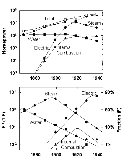
Figure 1. Sources of Power for Mechanical Drives in the United States.Note: The upper panel shows the absolute horsepower delivered by each type and their sum. The lower panel shows the fraction (F) of the total horsepower provided by each type, according to a logistic substitution model.Data Source: Warren D. Devine, Jr., “From Shafts to Wires: Historical Perspective on Electrification,” Journal of Economic History 43 (1983): 347_372; Table 3, p. 351.
At first, steam preserved the layout of the factory. It simply provided more flexible and dependable mechanical energy. The small early steam engines usually operated individual devices. A leap forward came with the advent of the single, efficient, cen tral steam station to serve all the machinery inside a plant. Pulleys rotating above the heads of the workers provided power for their diverse machines via vibrating and clapping belts. But the network of beams, blocks, cords, and drums for transmitting t he steam power to the machinery on the floor encumbered, endangered, and clamored.
The electric motor drive, which emerged around 1890, revolutionized the layout of the factory. The first era of electrical systems commenced. The steam engine now ran an electric generator that penetrated the factory with relatively inconspicuous coppe r wires carrying electricity, which in turn produced mechanical energy at the point of consumption with an electric motor. Here was the seed of modern manufacturing. The electric motor drive permitted the factory machines to be moved along the production sequence, rather than the reverse.
One might suppose that the superior electric transmission, with a generator at one end and motors at each machine, would quickly supplant the old mechanical system. In fact, as Figure 1 shows, the process required fifty years. Resis tance was more mental than economic or technical. In 1905 the influential American historian and journalist Henry Adams chose the images of the Virgin and the dynamo around which to write his autobiography.4 The dynamo symbolized the dangerous, inhuman, and mindless acceleration of social change.
Power for the Region
By the time arcs and lamps emerged from Mr. Edison’s workshops, the generator could illuminate as well as grind, cut, and stamp. But the paradigm of the single generator for the single factory was soon superseded by the idea of a generator, or, better yet, a power plant, serving an entire community.
At first, electric companies were necessarily small. Technology for the transport of electricity particularly limited the scale of operations. The original Edison systems were based on low-voltage direct current (dc), which suffered drastic energy loss es over distance. Each piece of territory thus required its own company, and founding a new company meant filling a piece of territory or market niche.
Consider eastern Pennsylvania, a coal-and-steel region where some of the earliest Edison utilities began (Figure 2). Entrepreneurs swarmed the area to spread the successful innovation. About 125 power-and-light companies were establ ished between the middle 1880s and early 1920s, with 1897 being the year of peak corporate fertility. The rush to form companies was a cultural pulse, diffused by imitation.5
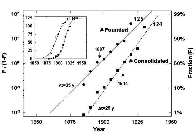
Figure 2. Founding and Consolidation of Electric Companies in the United States.Note: The main figure presents the two sets of data shown in the inset panel fitted to a linear transform of the logistic curve that normalizes each process to 100 percent, with estimates for the duration of the process, its midpoint, and saturation l evel indicated.Data Source: Pennsylvania Power and Light, Corporate History in nine volumes, Origin and Development of the Company, vol. 1, Allentown, Pa., 1940.
The evolution of technology to transport electricity, combined with the increase in the density of consumption (kW/km2), made higher transmission voltages economical and progressively coalesced companies. The key technology, first explored i n the 1880s by the inventor Nikola Tesla, was alternating current (ac), which could be raised in voltage through transformers and then transmitted long distances with low losses. The merger wave crested in 1914. By 1940 the resulting process left only Pen nsylvania Power and Light in operation.
When companies cover a geographical space, their natural tendency is to coalesce, like soap bubbles, especially if a technology permits the larger scale physically and encourages it economically. Several non-technical factors, including government and consumer fears about monopoly, can set limits on scale. Early in the century, Samuel Insull’s “electricity empire,” centered in Chicago, evoked public regulation, which became normal for the industry. Rapid growth and change usually elicit external regula tion. Still, the systems grow in the long run, as we shall see.
In the provision of electric power, the overriding independent variable is spatial energy consumption. Its increase leads to higher-capacity transport lines using higher voltage, making it possible to transport energy over longer distances with generators having higher power. This “higher and higher” game led the United States from the 10-kilowatt generator of Edison to the 1-gigawatt generators of today, one hundred thousand times larger.6
In fact, the expansion divides into two eras, as we see in Figure 3, which shows the evolution of the maximum line capacity of the US electric system. For the line-capacity indicator, we take over time the square of the highest volt age that is operational. Although various factors lower actual line capacity in practice, this indicator provides a consistent measure of power capacity for analysis of long-term trends.7 The maximum line capacity grows in two waves, one centered in 1921 and the second fifty-four years later in 1975.
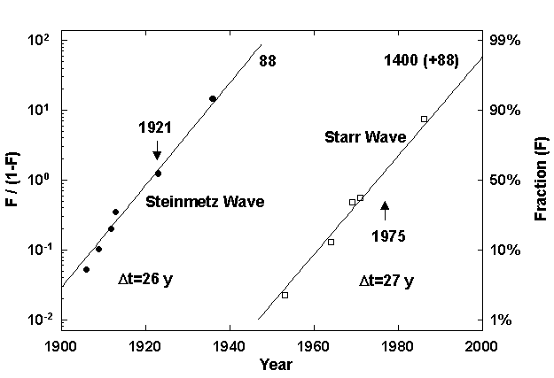
Figure 3. Capacity of Top US Power Lines.Note: The units are kV2/1,000-a rough measure of power capacity. This figure as well as Figures 4, 6, and 8 show a two-phase process analyzed as a “bi-logistic” normalized with a l inear transform. In essence, one S-shaped growth curve surmounts another. The actual values are the sum of the two waves, once the second wave is underway. See Perrin S. Meyer, “Bi-logistic Growth,” Technological Forecasting and Social Change 47 (1 994): 89_102.Data Source: Edison Electric Institute, Washington, D.C.
We label the first wave “Steinmetz,” for Charles Proteus Steinmetz, the founding leader of the engineering department of the General Electric Company (GE) and a symbol of the fruitful interaction of mathematical physics and electrical technology.8 Following the pioneering work of Tesla, Steinmetz began investigating the problems of long-distance transmission and high-voltage discharges around 1905. The spectacular success of GE in subsequent decades testifies to the timel iness of Steinmetz’s innovations. New alternating-current systems and related gadgets made huge profits for GE and the other leading equipment supplier, Westinghouse, and incidentally killed many small-scale utilities, as in Pennsylvania.
The second pulse of growth in line voltage reaches a temporary ceiling at about 1.5 megavolts. Interestingly, the stretches of innovative activity, as measured by the interval to achieve 10 to 90 percent of the system development, cover only about half the time of electricity’s waves of growth. Two to three decades of rapid expansion are digested in a comparably long period of stability and consolidation, a frustrating cycle for engineers. Again the limit may not be technical or economic, but social. S ociety tailors the expanded system to fit its norms for safety and harmony. One constraint is available rights-of-way, which are very limited at present.
Because the area of the United States is constant and filled by the electrical network, total generating capacity approximates the spatial density of consumption. The growth in installed generating capacity also splits into two pulses, centered around 1923 and 1971 (Figure 4). At peak times operators experience the most rapid change and customers suspect the operators’ ability to handle it. During the second wave, annual growth in consumption peaked in the 1950s and 1960s at more th an 10 percent per year for many US utilities. The system in the Northeast blacked out one day in November 1965, prompting regional power pooling arrangements. To address concerns about the reliability of the entire network, the industry consorted to form the Electric Power Research Institute, which opened its doors in 1973 under the leadership of Chauncey Starr, for whom we name electricity’s second wave.9
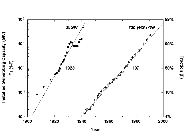
Figure 4. Installed Electric Generating Capacity in the United States.Data Source: US Bureau of the Census, Historical Statistics of the United States (Washington, D.C.: US Bureau of the Census, 1978); and US Bureau of the Census, Statistical Abstract of the United States (Washington, D.C.: US Bureau of th e Census, 1978, 1981, 1984, 1986, 1989, 1991, 1992, 1994).
The current pulse of growth in US generating capacity reaches a ceiling around 765 gigawatts. The actual system growth has exceeded 90 percent of the niche, which in our view explains the recent slowdown in the building of power plants, nuclear or othe r, in the United States. The system anticipated the growth in demand that is tuned to economic development and technological diffusion, boxed into the long, roughly fifty-year economic cycles that have characterized the last two hundred years.10 At the end of the cycles, demand lags and overcapacity tends to appear.
Will the higher-and-higher game resume? In both line voltage and generating capacity, the growth in the second electrical wave exceeded the first by more than an order of magnitude. If the pattern repeats, the increase in electricity consumption will l ead to ultra-high voltage lines (for example, + 2 megavolts) with higher capacity (for example, 5 or 10 gigawatts) and continental range. The great advantage of continental and intercontinental connections is that standby reserves and peak capacity can be globalized. The worldwide load would be smoothed over the complete and immanent solar cycle. Generators could also become very large, with according economies of scale.
If the system evolves to continental scale, the much-discussed superconductivity at room temperature might not revolutionize transmission after all. Energy lost in transport and distribution is a stable 10 percent, a huge amount in absolute terms, but too small to change the basic economics if 2-megavolt lines cover the continents. Superconductivity could, however, bring about a revolutionary drop in the size of machinery, thereby permitting the construction of units of larger capacity.
Continental scale surely means increased international trade in electricity. All territory looks the same to electricity. If available technology is employed, electricity will stream across borders despite the political barriers that typically impede t he easy flow of goods and ideas. Today Europe exchanges electricity almost freely. Italy buys from France the equivalent production of six 1-gigawatt nuclear reactors either via direct high-voltage lines or through Switzerland. Electricity trade could for m a significant component of international payments over the next fifty to one hundred years, requiring reorganization and joint international ownership of the generating capacity. Electricity trade between Canada and the northeastern United States alread y elicits attention.
Utilization and Capacity
The utilization factor of generation plants counts heavily in the economy of the system and indicates the quality of its organization. The US electric industry searched successfully between 1910 and 1940 for efficient organization, notwithstanding the Great Crash of 1929, as the average annual utilization climbed from two thousand to above four thousand hours, a utilization rate of about 50 percent (Figure 5). The rise owed to spatial integration and the reduction of reserves conseq uent to the introduction of high-capacity transport lines with increasing operating voltage as well as the coordination of network dispatch to use plants more effectively.
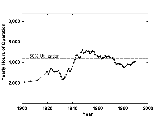
Figure 5. The Rate of Utilization of US Electric Generating Plants.Data Source: US Bureau of the Census, Historical Statistics of the United States (Washington, D.C.: US Bureau of the Census, 1978); and US Bureau of the Census, Statistical Abstract of the United States (Washington, D.C.: US Bure au of the Census, 1978, 1981, 1984, 1986, 1989, 1991, 1992, 1994).
Since 1940 the system appears to have fluctuated around a utilization rate of 50 percent. Generators with low capital cost and high variable cost combine with base-loads plants with high capital cost and low variable cost to determine the current usage level. Although the utilization factor surely has a logical upper limit quite below 100 percent, even with high-voltage lines having continental reach, a 50-percent national average appears low, notwithstanding scorching August afternoons that demand ext ra peak capacity.
Breaking the 50-percent barrier must be a top priority for the next era of the industry. Otherwise, immense capital sits on its hands. One attractive way to make electric capital work around the clock would be to use plants at night. The mismatched tim ing of energy supply and demand existed when water power dominated. Pricing, automation, and other factors might encourage many power-consuming activities, such as electric steel-making, to go on the night shift. Nuclear heat, generating electricity by da y, could of course help to make hydrogen at night. The ability to store hydrogen would make the night shift productive.
The nearness of overcapacity in the electrical system also creates suspicion that forecasting within the sector has not been reliable. Analyses of projections of total electricity use made by the US Department of Energy and others fuel the suspicion. R eflecting a period when electricity consumption had doubled in spans of ten years, in 1978 federal officials projected an increase by 1990 from 2,124 terawatt hours to 4,142 terawatt hours.11 The actual level for 1990 was 2 ,807 terawatt hours.
Can we do better? Fitting the data for total utility electric use to our model with data through 1977 yields an estimated level of about 2,920 terawatt hours for the growth pulse now ending (Figure 6). Net generation in 1993 was 2,8 83 terawatt hours. Projecting electricity demand matters because it influences investments in capacity. Accurate projections might have lessened the pain for the utilities, which ordered and then canceled plants; the equipment suppliers, who lost the orde rs; and consumers, who ultimately pay for all the mistakes.
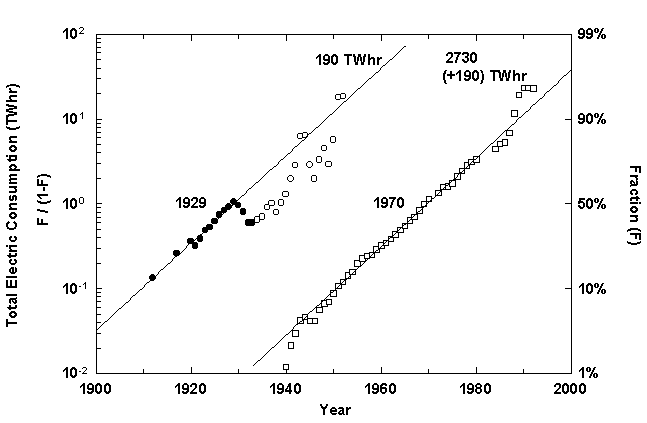
Figure 6. Total US Electric Consumption.Note: Here and in Figure 8 the empty circles indicate periods of overlap in the sequential growth waves. Assigning the exact values to each wave during the periods of overlap is somewhat arbitrary.Data Source: US Bureau of the Census, Historical Statistics of the United States (Washington, D.C.: US Bureau of the Census, 1978); and US Bureau of the Census, Statistical Abstract of the United States (Washington, D.C.: US Bureau of the Census, 1978, 1981, 1984, 1986, 1989, 1991, 1992, 1994).
Power for the Home
As suggested earlier, electricity is a spatial technology. Conquering a territory means connecting with potential users. We tend to think that almost everyone was connected soon after the first bulb was lit, but in fact the process extended gradually over fifty years and culminated even in the United States only in mid-century (Figure 7). Although slowed by the Great Depression, non-rural hookups reached 90 percent of the market by 1940. Rural areas joined the grid about one generat ion later than cities, reaching a midpoint of the process in 1943 versus 1920 for the townsfolk. This interval measures the clout of rural politicians, who secured subsidies for the costly extension of power lines to areas of low population density, as we ll as the conservatism of the countryside.
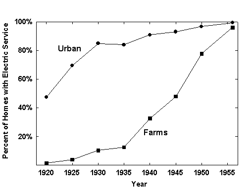
Figure 7. Percentage of US Homes with Electric Service.Data Source: US Bureau of the Census, Historical Statistics of the United States (Washington, D.C.: US Bureau of the Census, 1978).
The data further confirm that electricity’s first century has encompassed two eras. During the developmental spread of the system until about 1940, most electricity went for industry and light, substituting for other energy carriers in already existing market niches. In the second era, electricity powered new devices, many of which could not have performed without it, such as televisions and computers. Most of the new demand came in the residential and commercial sectors.
Average residential consumption has increased by a factor of ten since 1940 and appears in our analyses to saturate in the 1990s at about 10,000 kilowatt hours per year. One might say that the customer is the home, not the human. Home appliances have i ncreased by the tens and hundreds of millions: refrigerators, video-cassette recorders, vacuum cleaners, toasters and ovens, clothes washers and dryers, dishwashers, air conditioners, space heaters, and, more recently, personal computers, printers, and fa x machines.
We emphasize the residential because it is becoming the number-one consumer. Residential consumption has grown faster than other major sectors over the past decades and in 1993 overtook industrial consumption in the United States. The number of housing units has grown sevenfold in the United States since 1900, while the number of people has tripled, as residents per unit have declined and second homes increased. 12 As the second wave of electrification reaches its culmina tion, the residential share appears destined to plateau at about 35 percent of the total use of electricity, more than twice its share of the first wave. In a third wave of electricity, residential consumption may grow only at the same rate as overall con sumption, or, if life-styles continue to include more home space and reduced working time, at an even faster rate.13 Californians already spend more than 60 percent of all their time at home indoors.14 So do New Yorkers and Indians.
Cleaning the Human Environment
In the absence of electricity, we heat, light, and power our homes and workplaces with wood, coal, kerosene, oil, manufactured city gas, and lesser fuels. Electrification has thus meant a cleaner, safer, and healthier environment at the level of the en d-user, once protections against shock and other hazards were properly wired into the system. Dangers associated with open fires and smoke diminished. Better-ventilated homes and workplaces lessened exposure to influenza, pneumonia, tuberculosis, diphther ia, measles, whooping cough, scarlet fever, and other airborne threats. Modern refrigeration in homes, shops, trucks, and railroad boxcars reduced the numerous waterborne gastrointestinal threats.
Environmentally, electricity concentrates pollution at a few points. At these points we can deal with the problems or not. The main question then becomes: What is the primary energy source for the generation? The most wanted environmental culprit is ca rbon, and so the main environmental challenge for electricity may be summarized by the measure of the carbon intensity of electricity production, for example, the ratio of carbon by weight to kilowatt hours generated.15 In the United States, this ratio fell by half between 1920 and 1940, from about 500 metric tons of carbon per gigawatt hour produced to about 250. Since the 1940s, the US ratio has fallen below only about 200 metric tons per gigawatt hour and has remained ra ther flat in recent decades because coal has gained markets in electric power plants, offsetting efficiency gains in the operations of the plants as well as gains in terms of reductions that oil and especially gas would have contributed. Many other countr ies have continued to create more watts with fewer carbon molecules. The powerful underlying evolution of the energy system from coal to oil to natural gas to nuclear or other carbon-free primary sources will bring reductions.16 The world appears a bit past the middle point of a decarbonization process that will take another 150 years for completion. The United States will not long remain apart from the global movement.
Electricity production was originally based on coal alone. At present, it is the only outlet for coal. Even steel-making, which historically consumed a substantial fraction of coal (sometimes more than 10 percent), abandoned coal, dropping demand. Coal will fight hard to keep its last customer. Interestingly, electricity was never linked to oil, one of the other major transforming technologies of the twentieth century. Electricity and oil may now begin to compete seriously for the transport market, as we discuss later. Natural gas is already penetrating the electrical system thanks to the great flexibility, low capital cost, quick starts, and efficiency of gas turbines. At present, electricity remains the only product of the nuclear system. Approaching an energy system with zero emissions, about which all environmentalists dream, will require nuclear to diversify into the hydrogen-making business. The team of electricity and hydrogen can eventually solve all the problems of pollution at the level of th e end-user of energy.
Electrical systems can add visual pollution with their network of towers, wires, and poles. Militant Greens already dynamite pylons and will accept no new structures. New technologies can increase the capacity of the existing lines and diminish intrusi ons. In this regard, direct current, now ultra-high, may have a second life as a bulk carrier aided by relatively cheap electronics, such as thyristors, which are capable of transforming all types of units of electricity into all others. Burying power lin es might beautify the landscape, as well as lessen fears about the health effects of electromagnetic fields.
Feeding the Electrical System
A growing share of primary fuels generates electricity; again, two waves are evident (Figure 8). At the world level, the first centered in 1920 and the second in 1970. The present wave is saturating at close to 40 percent. For the U nited States, the current wave appears to have saturated at about the same level.
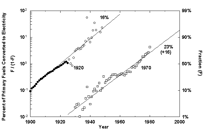
Figure 8. Percentage of World Primary Fuels Converted to Electricity.Data Source: Nebojsa Nakicenovic, personal communication, 1995.
Is there a limit to the fraction of fuels feeding into the electrical system? Many energy buffs postulate a ceiling at around 50 percent. A third era of electrical growth does seem likely to occur. Electricity is more flexible and fungible than hydroca rbon fuels. The innumerable devices of the information revolution require electrical power. The transport sector, which has remained largely reliant on oil, could accept more electricity. But the drawbacks are the inefficiencies and the costs of the trans formation.
Inefficiencies are eventually eaten up.17 A successful society is, after all, a learning system.18 In fact, perhaps the greatest contribution of the West during the past three hundred year s has been the zeal with which it has systematized the learning process itself through the invention and fostering of modern science, institutions for retention and transmission of knowledge, and diffusion of research and development throughout the econom ic system. But learning may still go slowly when problems are hard.
The Six-Hundred-Year War for Efficiency
The degree of difficulty for society to learn about power and light shows quantitatively in the duration of the process improvements illustrated in Figure 9. Technologists fought for three hundred years to bring the efficiency of s team power generation from 1 percent in 1700 to about 50 percent of its apparent limit today. Electrical energy is glorified as the purest form of free energy. In fact, the heat value of other fuels when they burn also corresponds to free energy. Thus, th e thermodynamic limit of electric generators is 100 percent. Of course, it can be very difficult to reduce losses in combustion. Still, we may muse that during the next three hundred years efficiency will go to 99 percent.19 This long trajectory suggests that the structure upstream for power generation does not leave much room for spectacular breakthroughs.
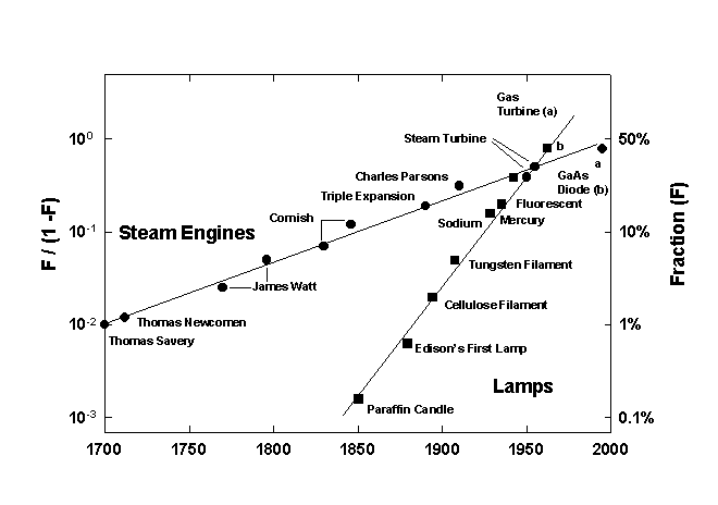
Figure 9. Improvement in the Efficiency of Motors and Lamps Analyzed as a Sigmoid (logistic) Growth Process. Note: Shown in a linear transform that normalizes the ceiling of each process to 100 percent. Main Sources of Data: for lamps, Encyclopaedia Britannica, 1964; for motors, Hans Thirring, Energy for Man (Bloomington, Ind.: Indiana University Press, 1958).
Still, 70-percent efficiency can be eyed as the next target, to be achieved over fifty years or so. Turbosteam plants with an efficiency of about 60 percent have been constructed. Although further gains in this regard appear limited, the massive diffus ion of highly efficient turbine technology is sure to be a lucrative and influential feature of the next fifty years or so. Fuel cells, avoiding the free energy loss almost inevitable in the combustion process on which turbines rely, may well lead to the even higher efficiencies. Electrochemistry promises such technology but mentally seems more or less still stuck in Edison’s time. Perhaps solid-state physics can produce the insights leading to the needed leap forward as specialists in this field become m ore interested in surfaces, where the breakthroughs need to occur.
At the 70-percent level of efficiency, an almost all-electric distribution of primary energy looks most appealing. The catch is the load curve, which seems likely to remain linked to our circadian rhythms. In Cole Porter’s song lyric, we hear “Night an d day, you are the one”; but in energy systems night still dims demand and means expensive machinery remains idle. Even in cities famous for their nightlife, nocturnal energy demand is only one-third of the daytime requirement. The ratio of day to night a ctivity does not seem to have changed much. The ancients actually spent considerable time awake at night, despite miserable illumination. The fine old word “elucubrate” means to work by the light of the midnight oil, according to the Oxford English Dic tionary.
Even if most humans continue to sleep at night, we have pointed out earlier that their energy-consuming machines can work nocturnally. In fact, remote control and the shrinking work force required to operate heavy industry ease the problem. So, too, wi ll linking parts of the globe in sun and shade, summer and winter.
Still, we should clearly look further for efficiency gains. Much large electrical machinery is already so efficient that little or no gain is to be expected there. But a discontinuous step could yet come in the progress of machinery. Superconductivity, when it permits high magnetic fields, can lead to compactly designed motors with broad applications and very low energy losses. The proliferation of numerous micro-machines will of course tend to raise electricity demand, partially offsetting the efficie ncy gains they offer. The miniaturization of circuits and other aspects of computing systems in the past two decades shows how powerfully reducing the size of objects can increase their applications and numbers.
The Splicer
In proposing a more general solution we need to introduce another consideration, namely, reliability. The main drawback of an electrical system is that it permeates the web of social services, so that a breakdown, even for a few hours, can bring traged y. A defense against this vulnerability, as well as a means of addressing cyclical loads, could come with the diffusion of multipurpose minigenerators at the level of individual consumers. In effect, we would delegate base load to the global system, leavi ng peaking and standby to a new multipurpose household appliance. Multipurpose means the device could produce heat, electricity, and cold on demand.
Such combined thermal, electric, and cooling systems, which we will call “splicers,” are under development. Attempts so far, such as the FIAT TOTEM, have been unsuccessful, in part because the marketed models lack the basic characteristic of zero ma intenance required by household gadgets. Still, the scheme is appealing, both functionally and economically. The Japanese are doing a sizable amount of research and development in what appears to be a promising direction: stirling engines with free-fl oating pistons and a power output of a few kilowatts. The machines are maintenance-free, silent, and can compress fluids for the heating and cooling cycles on top of producing electricity with linear oscillating generators. The models described in the lit erature are powered by natural gas.
In conjunction with a clean gas distribution system, the penetration of the splicer as a home appliance over the next fifty years could revolutionize the organization of the electrical system. The central control could become the switchboard of million s of tiny generators of perhaps 5 kilowatts. Electric utilities might initially abhor the technology that brings such functional change, but already some plan to use it. One attraction is that the final user immediately pays the capital cost.
In any case, the breakthroughs may come instead on the side of the consumers. A number of well-known machines and appliances need technological rejuvenation, as efficiencies are systematically low. And new machines need to be invented. At a high level of abstraction, human needs are invariant: food, clothing, shelter, social rank, mobility, and communication (a form of mobility where symbols move instead of persons or objects). Let us guess the shape of the new machines in the areas of vision and warmt h.
Efficient Vision
Illumination, the first brilliant success of electricity beyond powering the workshop, provides a good example. Breaking the rule of the night is an old magical dream. The traditional tools-oil lamps, torches, and candles-were based on a flame w ith relatively low temperature and small amounts of incandescent soot to emit the light. They performed the task poorly (see Figure 9).20 The typical power of a candle is 100 watts, but the light efficiency is less than 0.1 percent.
Electricity fulfilled the dream, almost from the beginning, with arc lights, whose emitting source was solid carbon at temperatures of thousands of degrees centigrade.21 The light was as white as the sun, and efficiency reached about 10 percent. The technical jump was enormous. Theaters, malls, and monuments were lavishly illuminated. People were seduced by the magic. Amusement parks such as Luna Park and Dreamland at Coney Island in New York drew millions of paying visi tors to admire the architectural sculptures of light.
Edison’s 1879 incandescent lamp was a trifle inferior to the arc in light quality and efficiency but was immensely more practical. Symbolically, in 1882 the New York Stock Exchange installed three large “electro-liers,” new chandeliers with sixty-six e lectric lamps each, above the main trading floor. The exhibition of the power to break the night came first and dramatically. Penetration of the technology came later and, as usual, slowly. US cities, as shown earlier, achieved full illumination only abou t 1940.
The period from 1940 to 1995 can be called a period of consolidated light. Lamps became brighter and efficiency rose. To the human eye, the quality of the light may actually have worsened with the spread of fluorescents. With laser light, which has ter rible visual quality now, we may approach theoretical efficiency, though actual lasers remain inefficient. Will that be the light at the end of the tunnel?
To return to basics, we illuminate in order to see in the dark. Illumination has no value if nobody looks. Arriving in a town at night, we always see the roads brightly lit and empty, so we know of waste. The marvels of the 1980s, electronic sensors an d computer chips, can already scan rooms and streets and switch the lights off if no one is present. The watt-watch can help, but we can go further.
Sophisticated weapons systems-those mounted in helicopters, for example-feel the thumb of the pilot, observe his eyes, and shoot where he looks. A camera-computer in a room can watch the eyes of people present and illuminate only what they watch. Phase d arrays, familiar in sonars and radars and developed now for infrared emitters, are certainly transportable into the visible range and can create sets of beams that are each directed to a chosen point or following a calculated track. The apparatus might now look baroque, but with miniaturization it could be concealed in a disk hanging from the ceiling of a room. Such a gadget appears to be the supreme fulfillment, illuminating an object only if a human gazes upon it.
But recall again that the objective is not to illuminate but to see. We illuminate because the eye has a lower limit of light sensitivity and, in any case, operating near such a limit is unpleasant. The military has developed complicated gadgets by whi ch scanty photons from a poorly illuminated target are multiplied electronically to produce an image of sufficient luminosity. The principle is good; the machine is primitive. If photons flowing in an energized medium (such as an excited laser crystal) mu ltiplied in a cascade along the way while keeping frequency and direction, we would have invented nightglasses, the mirror image of sunglasses.22 We could throw away all sorts of illuminating devices. A few milliwatt s of power would be enough to brighten the night.
Efficient Warmth
The largest part of energy consumed in the home is used for temperature control. Space heating accounts for 60 percent or more of total residential energy use in many developed countries. Heating a home is a notably inelegant process from a thermodynam ic point of view. We use pure free energy (electricity or fossil fuels) to compensate for a flow of energy from inside to outside having an efficiency according to the Second Law of Thermodynamics of about 3 percent if the difference in temperature is 10< SUP>oC. Heat pumps solve the problem conceptually, but they see temperatures inside their heat exchangers and consequently overwork.23 Moreover, operating on electricity generated upstream, they already invite inefficiency into the endeavor.
Consider a radically different proposal. Windows are the big leaks, even when the glazing is sophisticated and expensive. Why not use window panes as thermoelectric devices, not to carry heat uphill but to stop heat from sledding downhill, that is, as heat-flux stopping devices?
Thermoelectric generators are usually seen as machines to make electricity by using the principle of the thermocouple. However, the device is reversible: by passing electricity through the machine, heat can be moved uphill. Several decades ago refriger ators were proposed using this principle on the basis of its great simplicity, although efficiencies are low. The old scheme for refrigerators could be revised in view of new thermoelectric materials and given suitably competitive objectives.
The basic idea is that electrodes on the inner and outer surfaces of the windowpanes can be made of conductive, transparent glasses. Glass made of zinc oxide might be sufficiently conductive. Voltages across the glass would be very low-volts or fractio ns of volts. Holding a temperature differential with zero flux would be more efficient energetically than putting heat (electrically!) into a house to balance the outgoing flux.
Electric Motion
So far we have looked at examples where efficiency wins, and net demand for power grows, only if the human population and its use of devices increase faster than efficiency. Now let us look at one example where a large new market might emerge, matching the ultra-high voltage lines and continental connections.
Toward the end of the last century electric motors for vehicle engines attracted much inventive action. Edison and Ferdinand Porsche produced sophisticated prototypes. The idea flopped on the roads but succeeded on the rails. Electric trams clamored th rough American and European cities, helped create suburbs, and in some cases connected cities. After 1940 most of the system was rapidly dismantled, largely because the trams could not match buses and cars in flexibility or speed. The mean velocity of tra nsport keeps increasing through the progressive substitution of old technologies with new, faster ones. For France, the increase in the average speed of all machine transport has been about 3 percent per year during the last two centuries. Urban and subur ban railways have a mean speed of only about 25 kilometers per hour, including stops. Cars have a mean speed on short distance trips of about 40 kilometers per hour. The latest in the series are airplanes, with a mean speed of 600 kilometers per hour. Air planes will provide most of the increase in mean speed over the next fifty years.
Electric trains succeeded in Europe and Japan for the densely trafficked lines and still operate today. They have decent acceleration and speed compared with diesels. But most trains are not fast; the inclusive travel time on intercity rail journeys is only about 60 kilometers per hour. The fastest trains, the French trains à grande vitesse (TGVs), are electric. The question for trains is how to compete with cars on one side and with airplanes on the other. Electricity probably cannot com pete with hydrogen for propulsion of cars and other light vehicles.
The great market challenge for the current generation of fast trains, with top speeds of 400 kilometers per hour, is the short distances of less than 100 kilometers along which cars congest and airplanes cannot compete. The present configuration of air ports and airplanes are high-speed but low-flux machines. TGVs could prove extremely competitive in the intense shuffling of commuters and shoppers within these distances. A cursory review of Europe reveals about 5,000 kilometers of intercity links fittin g the constraints of a 100-kilometer distance and high potential passenger flux.
Fast trains consume more or less the same amount of primary energy per seat-kilometer as a turboprop plane24 or a compact car. From the power point of view, a running TGV absorbs about 10 kilowatts per seat. The mean pow er demand of the proposed 5,000-kilometer system of TGV trains for commuters and shoppers would be around 6 gigawatts, with a peak of probably 10 gigawatts. If the concept is successful, this form of transport will be an important consumer of electricity, but it will take at least fifty years to become fully implemented.
To go to very high passenger fluxes over longer distances, one would need to go to aerial configurations of which even the most daring air-transport planners do not chance to dream: flocks of airplanes of five thousand passengers each taking off and la nding together like migrating birds.
For intense connections linking large cities with peak fluxes around ten thousand passengers per hour, a solution is emerging that matches system requirements: the magnetically levitated (maglev) train operating in a partially evacuated tube or tunnel. In fact, Swiss engineers have developed the concept of a vacuum version of maglevs in part to reduce drastically the tunnel boring expenses, which in Switzerland would account for at least 90 percent of the cost in a conventional layout. 25 To handle the shock wave from a high-speed train, a tunnel normally needs a cross section about ten times that of the train. In addition to narrowing greatly the tunneling requirement, the partial vacuum greatly reduces friction, making speed cheap and thus expanding the operational range of the train.
When operated at constant acceleration-for example, 5 meters per second or 0.5 g (the force of gravity), about what one experiences in a Ferrari sports car-maglevs could link any pair of cities up to 2,000 kilometers apart in fewer than twenty minutes. Consequently, daily commuting and shopping become feasible. Such daily trips account for 90 percent of all travel and are controlled by the total human time budget for travel of about one hour per day. With fast, short trips cities can coalesce in functi onal clusters of continental size. City pairs spaced less than 500 kilometers or ten minutes apart by maglevs, such as Bonn-Berlin, Milan-Rome, Tokyo-Osaka, and New York-Washington, would especially benefit.
Part of the energy consumption of vacuum maglevs overcomes residual friction; an economic balance must be struck between the friction losses and the pumping power to keep the vacuum. Part regenerates the electromagnetic system that pushes and pulls the trains.26 The power per passenger could roughly correspond to that of a large car, although these trains may travel at a mean speed of 3,000 kilometers per hour.
The great advantage of the constant acceleration configuration for maglevs is that the energy required for each length of track is constant and could be stored, perhaps magnetically, in the track itself. Power demand is proportional to train speed and moves into the gigawatt range in the central section; however, with local storage (a few kilowatt hours per meter) the external electric power networks would see only the need to make up losses. Even assuming 90-percent efficiency, these would not be negl igible. One hundred trains per hour would demand 1 gigawatt for the single line on which they operated.27 The Swiss system has a final potential of five hundred trains per hour, which would require 5 gigawatts-about one-thi rd of current installed Swiss generating capacity.
The first long-distance maglev will probably run in about five to ten years. Berlin-Hamburg is under construction. The penetration of the technology will be gradual, as major infrastructural technologies always are. In fact, the next fifty years will p robably be used largely to establish the feasibility, chart the maglev map, and prepare for the big push in the second half of the twenty-first century. In the long run, maglevs may establish several thousand kilometers of lines and become one of the most important users of electricity. A maglev trip per day becomes a few thousand kilowatt hours per year per person. If India and Eastern China join life in this superfast lane, the picture of a globally integrated, high-capacity electrical system begins to cohere.
Conclusions
The long economic cycles that seem to affect all parts of social and economic life constitute a good frame of reference for the development of the electrical system in terms of technology, territorial penetration, birth and death of enterprises, and in tensity of use. Our examples suggest this is true for the United States and globally.
Two waves of electrification have passed through our societies. In the first, the United States attained system saturation in the 1930s at about 1,000 kilowatt hours annual consumption per residential customer, 200 gigawatt hours of total annual use, 4 0 gigawatts of installed capacity, and 20 percent of primary fuels producing electricity. In the second wave, we have reached 10,000 kilowatt hours per residential customer, 3,000 gigawatt hours of total use, 800 gigawatts of installed capacity, and about 40 percent of fuels producing electricity.
The fact that the patterns of temporal diffusion and growth are followed makes it possible to fit dynamic equations to the time series of facts and then compare them for consistency. This operation indicates that the 1990s are the season of saturation, which includes the experience of overcapacity or, alternately, underconsumption. Such phases are not uncommon for various branches of the industrial system, as managers tend to assume that growth characteristics of boom periods will extend into recession s, while consumers cut corners.
In the short term, total energy and electric energy consumption may continue to grow at a slower rate than overall economic activity. One interpretation is that during the expansion period of the long cycles the objective is growth, while during the re cessive period the objective is to compete, shaving costs here and there and streamlining production. The savings include energy. Meeting goals pertaining to environmental quality and safety further tighten the system.
A new cycle formally beginning in 1995 started the game again, although the effects of the restart will not be particularly visible for a few years. Minima are flat. Looking at the cycles from a distance to grasp the general features, one sees the peri ods around their ends as revolutionary, that is, periods of reorganization-political, social, industrial, and institutional. We are evidently at this conjunction, and the electrical system will not escape it.
When the electrical system served the village, a complete vertical integration was inevitable. Regional coverage, the preferred scale of the past fifty years, also favored such integration. With the expansion to continental dimensions, a shift in respo nsibilities may make the system more efficient, agile, and manageable. The typical division is production, trunk-line transport, and retailing, with different organizations taking care of the pieces and the market joining them. The experiments in this sen se now running in Great Britain, Australia, and other countries can be used as a test bed to develop the winning ideas.28
Apart from various economic advantages and organizational complications, the use of splicers on a large scale-untried to date-may bring an almost absolute resiliency, as every subset of the system may become self-sufficient, if temporarily. The electri cal system should also become cleaner, as it intertwines more closely with natural gas and probably nuclear energy, thus furthering decarbonization. A sequence of technical barriers will appear, and thus the process of systematic research and innovation w ill continue to be needed; it will produce timely results.
In fact, our analyses suggest that rates of growth of technology tend to be self-consistent more than bound to population dynamics. Population, however, defines the size of the niche in the final instance. Thus a key question is, how long will it take to diffuse Western electric gadgetry to the 90 percent of the world that is not already imbued with it? The gadgetry keeps increasing. Followers keep following, if more closely. Based on historical experience, diffusion to distant corners requires fifty t o one hundred years. Even within America or Europe, as we have seen, pervasive diffusion takes that long for major technologies. So most people may have to wait for most of the next century to experience nightglasses, splicers, and maglevs. These devices may be largely features of a fourth wave of electrification, while the spread of the profusion of information-handling devices dominates the third wave that is now beginning.
Considered over centuries and millennia, the electrical adventure is deeper than a quest for gadgets. In 1794 Volta demonstrated that the electric force observed by Luigi Galvani in twitching frog legs was not connected with living creatures, but could be obtained whenever two different metals are placed in a conducting fluid. Today we use electricity to dissolve the difference between inanimate and living objects and to control and inspire the inanimate with more delicacy than Dr. Frankenstein. Introd ucing electricity into production raised the rank of workers from sweating robots to robot controllers. The process can be generalized, with humanity-at leisure or at work-giving orders to its machines by voice or a wink of the eye.
This ancient aspiration for action at a distance and direct command over the inanimate will drive invention, innovation, and diffusion for hundreds of years more; we come full circle to the elektron of the ancient Hebrews and Greeks.
Acknowledgments
We thank Perrin Meyer, for research assistance and figure preparation, as well as Arnulf Grübler, John Helm, Eduard Loeser, Nebojsa Naki¬enovi¬, and Chauncey Starr.
Endnotes
1“Oh subtle fire, soul of the world, / beneficent electricity / You fill the air, the earth, the sea, / The sky and its immensity.” Quoted in Robert Darnton, Mesmerism and the End of the Enlightenment in France (Cambridge, Mass.: Harvard University Press, 1968), 29.
2Edgar Allan Poe, The Science Fiction of Edgar Allan Poe (New York: Penguin, 1976).
3For general histories of electrification, see Thomas P. Hughes, Networks of Power: Electrification in Western Society (Baltimore, Md.: Johns Hopkins University Press, 1983); Richard F. Hirsch, Technology and Transformation in the American Electric Utility Industry (Cambridge: Cambridge University Press, 1989); David Nye, Electrifying America (Cambridge, Mass.: MIT Press, 1990); Wolfgang Schivelbusch, Disenchanted Night: The Industrialization of Light in the Nineteenth Century (Berkeley, Calif.: University of California Press, 1988); and Sam H. Shurr, Calvin C. Burwell, Warren D. Devine, Jr., and Sidney Sonenblum, Electricity in the American Economy: Agent of Technological Progress (Westport, Conn.: Greenwood Press, 1990). For data and information on the early history of energy and electricity, see H. D. Schilling and R. Hildebrandt, Primarenergie-Elektrische Energie, Die Entwicklung des Verbrauchs an Primarenergietragern und an Elektrischer Energie in der Welt, in den USA und in Deutschland seit 1860 bzw. 1925 (Essen: Vertrag Gluckauf, 1977).
4Henry Adams, The Education of Henry Adams: An Autobiography (Boston, Mass.: Massachusetts Historical Society, 1918; reprinted Boston, Mass.: Houghton Mifflin, 1961).
5Such diffusive processes are well fit by the logistic equation, which represents simply and effectively the path of a population growing to a limit that is some function of the population itself. For discussion of applications of logistics, see Nebojsa Nakicenovic and Arnulf Grübler, eds., Diffusion of Technology and Social Behavior (Berlin: Springer, 1991). On the basic model, see S. Kingsland, “The Refractory Model: The Logistic Curve and the History of Population Ecology,” Quarterly Review of Biology 57 (1982) : 29-52.
6A kilowatt (kW) is 1,000 watts; a megawatt (MW) is 1,000,000 W; a gigawatt (GW) is 1,000 MW; a terawatt (TW) is 1,000 GW. US generating capacity was 735 GW in 1990.
7Power is equal to V2/R, where V is voltage and R is resistance.
8John Winthrop Hammond, Charles Proteus Steinmetz: A Biography (New York and London: The Century, 1924).
9Chauncey Starr, “A Personal History: Technology to Energy Strategy,” Annual Review of Energy and the Environment 29 (1995): 31-44.
10Cesare Marchetti, “Fifty-Year Pulsation in Human Affairs: Analysis of Some Physical Indicators,” Futures 17 (3) (1986): 376-388.
11For an analysis of electricity projections, see Charles R. Nelson, Stephen C. Peck, and Robert G. Uhler, “The NERC Fan in Retrospect and Prospect,” The Energy Journal 10 (2) (1989): 91-107.
12See Lee Schipper, “Life-Styles and the Environment: The Case of Energy,” Dædalus 125 (3) (Summer 1996).
13Jesse H. Ausubel and Arnulf Grübler, “Working Less and Living Longer: Long-Term Trends in Working Time and Time Budgets,” Technological Forecasting and Social Change 50 (3) (1995): 195-213.
14Peggy L. Jenkins, Thomas J. Phillips, Elliot J. Mulberg, and Steve P. Hui, “Activity Patterns of Californians: Use of and Proximity to Indoor Pollutant Sources,” Atmospheric Environment 26A (12) (1992): 2141-2148.
15Sulfur and other emissions from power plants also cause ills, but these have proven to be largely tractable. See Nebojsa Nakicenovic, “Freeing Energy from Carbon,” Dædalus 125 (3) (Summer 1996).
16Jesse H. Ausubel, “Energy and Environment: The Light Path,” Energy Systems and Policy 15 (3) (1991): 181-188.
17N. Nakicenovic, L. Bodda, A. Grübler, and P.-V. Gilli, Technological Progress, Structural Change and Efficient Energy Use: Trends Worldwide and in Austria, International Part (Laxenburg, Austria: International I nstitute for Applied Systems Analysis, 1990).
18Cesare Marchetti, “Society as a Learning System,” Technological Forecasting and Social Change 18 (1980): 267-282.
19While Carnot efficiency (now about 60 percent) limits heat cycles, fuel cells do not face such a limitation, as they are not based on heat cycles.
20Gaslight, with a mantle with rare-earth elements, was a superior source of bright light for a period.
21The plasma struck between the two carbon electrodes also emits.
22Sticking to monochromatic light, a ray proceeding in a resonantly excited medium stimulates emission and becomes amplified. Amplification is relatively small with present devices; hence the ray must travel up and down betwe en mirrors. But no physical law limits amplification to such low levels. Semiconductor lasers, pumped by electric voltage, might hold the solution. In a second stage, they should also operate for a number of colors.
23The equivalent free energy of heat flowing out of a building is measured through the temperatures inside (T1) and outside (T2) in kelvin and is (T1-T2)/T1. In the case of a heat pump, due to temperature drops in the heat exchanger, it pumps heat from a temperature lower than T2 into a temperature higher than T1.
24For example, airplanes of the type ATR-42 or Dash.
25R. Nieth, W. Benoit, F. Descoeudres, M. Jufer, and F.-L. Perret, “Transport interregional à grande vitesse-Le Project SWISSMETRO,” Ecole Polytechnic Federale de Lausanne, 1991.
26We can calculate the amount of energy circulating in the system for a maglev with constant acceleration operating over a distance of 500 kilometers. A train of 200 metric tons accelerating at 0.5 g has a pull force (drag) of 1,000 kilonewtons, which over a stretch of 500 kilometers corresponds to 5 x 10¹¹ joules, or approximately 140,000 kilowatt hours. A mean loss of 10 percent would require 14,000 kWh for one thousand seats, or 14 kWh per seat over 500 km. This would correspond to 84 kW per passenger at a typical trip time of 10 minutes (e.g., Bonn to Berlin).
27For example, fifty trains might operate in each direction, spaced one minute apart. They can start from different stations or lanes. One per minute would be the frequency in the neck of the tunnel.
28For discussions of models of organizational change in the electricity industry, see Judith B. Sack, research memorandum series on “Global Electricity Strategy” (New York: Morgan Stanley), especially “The Darwinian Theory of Distribution” (12 December 1995), and “An Interrelated World” (29 February 1996).
Jesse H. Ausubel is Director of the Program for the Human Environment at The Rockefeller University.
Cesare Marchetti is an Institute Scholar at the International Institute for Applied Systems Analysis in Laxenburg, Austria.
Graphical representation of the world population growth
Human Population Dynamics Revisited with the Logistic Model: How Much Can Be Modeled and Predicted?
The following pages contain the full text and figures of an article which first appeared in the journal Technological Forecasting and Social Change, published by Elsevier Science Inc., New York, NY. Posted with permission.
Introduction: Runaway Growth or Slow Implosion?
As Charles Darwin said, in the struggle for life number gives the best insurance to win [1]. The Bible (Genesis 22:17) records that when God wanted to boost the elected ones, he promised that they would become more numerous than the grains of sand on the sea shore (i.e., >>1012).
In fact, world population since the mid 20th century has grown by about 2% per year, a rate that doubles the population in roughly 35 years. Actual data fitted over five centuries with reasonable equations show that the secular rate of growth kept increasing until around 1970, leading, at least from a mathematical point of view, to an infinite population in a finite time (Figure 1). (See [2] for a numerical history and [3] for an infinite prediction.) Such growth worries environmentalists and many others and leads to a first question: Where is the world population moving?
A second worry occupies rich, mostly white populations, in particular Europeans. The anxiety of their politicians and demographers (and the Pope) roots in the fact that on average a European woman now bears only about 1.4 children along her fertile span. To preserve a population, the rate should be around 2.1. The gap means that European populations are slowly imploding. An “oldies” boom preserves numbers for a while but empties society of the vis vitalis, the vital force carried by youth. Thus, a second question: Where is the population of the advanced industrialized nations moving?1
Two mechanisms control the size of a population: life expectancy at various ages and the fertility rate. (Migration also affects the size of local populations, but we will not consider it here.) For both death and birth, demographers still are searching for working models, that is, numerical models corresponding to theory whose parameters are set by independent data and whose results pass the test of conforming to still other data. (See [5] for a classic introduction to demography; [6] for a severe critique of progress a decade later; and [7, 8] for the current state of affairs.) The absence of working models means that the demographers cannot forecast the evolution of either life expectancy or fertility. Lee and Tuljapurkar, for example, state: “Doubtless the most important source of error in population forecasts is uncertainty about future [fertility] rates, because these rates are changing over time in ways that so far have been difficult to predict or even to explain after the fact”[9]. Thus, population predictions are based on numerical assumptions, or guesses, or “scenarios.”2
So far, demographic predictions tend to diverge from the real numbers after about 20 years. To give some examples, in 1951 the Population Division of the United Nations (UN) estimated that the world population in 1980 [10] would be between 2.976 and 3.636 X 10⁹. The use of four significant figures for a scenario is certainly worth a note. The number in 1980 was actually 4.45 x 10⁹. In 1986 the UN predicted 6 x 10⁹ for the year 2000. The 1995 world population is 5.7 x 10⁹. The UN mark will probably be reached in 1997. The UN 1992 prediction for 2150 is a la carte [11]. One can choose seven different world population levels placed between 4.299 x 10⁹ and 694.213 x 10⁹. However, the preference is for 11.543 x 10⁹. Unabated is the love for significant figures.
Predictions are always made with ifs. Because everybody seems scared by increasing human populations, fertility values are tamed in such a way-as to produce a maximum psychologically acceptable number of humans, usually between 1010 and 2 x 1010 by 2100. The reckoning date is well beyond the life expectancy of present politicians and demographers. These soothing predictions are obviously based on the if that current total fertility rates will fall everywhere to the conservation value of 2.1 (see Figure 6, later). As in weather forecasting, building the analysis from the bottom up becomes more and more complicated when one details to regions (and social status), and forecast results are not better.
Suffice it to say that the problem of the future size of humanity is unsolved. Whether the answer is unknown or unknowable, the problem partly lies in the methods, and no sign of breakthrough has appeared in the literature. Our response is to go back to the numbers and have a fresh look. We seek quantitative regularities to see whether it is possible to forecast with some internal logic where and when the growth will stop.
For both mortality and fertility all the mechanisms involved are regulatory and require social and cultural intervention. Because changes in culture and social behavior can be described by diffusive processes, basically captured in logistic equations (or their derivatives or sums), our fresh look will refuter the numbers along these lines. The fact that we can model with good precision over long periods several parameters usually looked at in charts in a qualitative way will show the strength of our method.
The use of the logistic model is widely established in many fields of modeling and forecasting [12, 13]. It has a controversial history in population ecology, a point to which we return near the end of this article. One of a family of density-dependent functions, the logistic law of growth assumes simply that systems grow exponentially under the constraints of an upper limit producing a typical S-shaped curve [14]. The three parameters of the logistic curve, which recur in our figures, are characteristic duration Dt, the limit K, and the midpoint tm. The characteristic duration Dtis the time needed for the curve to grow from 10% to 90% of the limit K. Appendix 1 offers a mathematical description of the logistic model.
There is obvious need for demographic statistics of reasonable quality and consistent definitions. See [2, 11, 15-28] for data sources. We also offer precise definitions of terms in the Glossary, Appendix 2. Shortcomings arise in several ways. For example, although local demographic registrations are of ancient origin and reliable, their patching up into national statistics may not be. African states may have made written records only recently. Changing cultural values affect what is recorded. Years for which detailed survey data are available are few and do not include all countries. In Appendix 3 we give some quantitative examples of the uncertainty associated, even in the present day, with fertility rates. Nevertheless, we believe that the long-run and comparative nature of our approach makes the analyses robust.
Our plan is to look first from the bottom up, using the logistic to model life expectancy and then, in much greater detail, fertility. When cases are intractable analytically, as modeling human population has been, the alternative is to look from the top down with phenomenological insights. The master case is that of thermodynamics, where a couple of well-centered axioms permitted almost two centuries ago the construction of a branch of physics unchallenged to date. Its analytical counterpart, statistical mechanics, took a full century to develop. In the case of demography, analysis of the aggregate behavior or niche started for animal populations in the mid-1800s. Before concluding, we briefly reapply the logistic model to the analysis of aggregate human populations with the help of some extra hindsight.
Modeling Life Expectancy
Life expectancy is an important parameter in defining the size of a population because for a given birth rate the number of people is proportional to it.
Life expectancy in the developed world started changing in about 1800, improving slowly. The maximum gains have been in reducing infant mortality, but octogenarians also gained a few years. Demographers and medical doctors still struggle to define the future of the process. A simple solution can be found by assuming that each of us is endowed with longevity by DNA. Dangers along the way impede reaching the final age. However, by removing the dangers through nutrition, hygiene, medicine, and various coatings and protections, finally one can reach an age corresponding to longevity.
Because the removal of the dangers is a process of social learning, the equation most apt to describe it is a logistic [29]. For a time, knowledge and experience enable people to gain years of life with increasing speed. Then the process slows as we near the limits of efficacy of our various strategies. In fact, evolution of life expectancy during the last two centuries can be precisely mapped using logistics. In Norway the gain in life expectancy at birth forms a neat logistic taking off at the 1% level in 1810 and eventually adding 39 years to the life of the new-born Norwegian child (Figure 2). The process is logistic at each age, with 20-year-olds eventually gaining 20 years, 50-year-olds 11, and 80-year-olds 3 (Figure 3). In fact, one can also map with a logistic the final gain versus age, as we have done for the Dutch population (Figure 4).
All such analyses show that in developed countries we are near a limit [30]. Barring genetically engineered defense against senescence, life expectancy for women will stay in the mid-80s and for men about 5 years less.3 Consequently, the effect of increasing life expectancy on population, which for a while has masked the decrease in fertility in some rich countries, will disappear.
For developing countries we have not attempted to analyze comparable trends because the series of credible population statistics are not long enough. We would expect similar results. The basic processes of social development are the same, though perhaps operating more rapidly than they did for the countries that industrialized early. In developing countries, increase in life expectancy will sum up quickly, boosting the size of their populations on top of the effect of fertility.
In the long term, life expectancy acts as a fixed multiplier on population and is thus much less important than fertility, which acts exponentially.
Modeling fertility
Reproduction is at the center of life. As Manfred Eigen showed in his seminal papers 30 years ago, survival is the axiom from which the mathematics of life can be deduced [31]. But survival in an abrasive context means starting again and again, i.e., reproduction. Being central to survival, reproduction naturally also occupies a central place in the thinking and action of human societies. However, species are normally endowed with excessive reproductive capacity to take care of critical transients and occasional opportunities. Where survival rates are high, as in birds of prey who have few natural enemies, total fertility tends to be low. A chick every year or two for each female can suffice. Animals with lots of hungry enemies and poor defenses, such as snails, tend to astronomical prolificity.
These generic observations may have trickled down into the concept that in humans the transition to lower mortality will lead to a fertility transition to replacement levels. Visual observation of mortality and nasality curves for many nations shows in fact that both fall starting in the latter part of the 19th century (as shown for Finland in Figure 5). The reported decrease in mortality typically precedes that of fertility.
The post hoc propter hoc is necessary, but rarely sufficient, to determine a causal relationship. The two phenomena can descend from the same cause. To give a whimsical but not impossible mechanism, eating peanut butter could increase health and inhibit fertility. The phenomena could also be completely unrelated. A famous chart shows the decreasing number of storks flying to Germany during the last 30 years, closely matching the number of children born, by a constant multiplicative factor.
Certainly decreasing the mortality of infants and the young before reproductive age reduces the need to produce many offspring. But the human species is endowed with excess fertility that had to be, and was, pruned even before the decrease in mortality that came after 1800, to fix a round reference date.
A free-wheeling human female can produce a dozen or more children during her fertile period. Although this number was fairly frequently reached in agricultural families up to 1900, most families stopped at much lower levels, say 4 children born. This essential fact means that fertility was always under control, helped in case of necessity by infanticide, a practice widely used up to our days [32]. In Western countries infanticide is mostly substituted by abortion, which is the same act at a different time. Because fertility has always been under control, we must ask then why people stop at one number instead of another and, whether the choice, probably made without explicit reasoning, can nevertheless be rationalized.
Some years ago a striking attempt at rationalization was made for India. It was observed that India had a mortality transition, but did not seem to have a marked fertility transition. The mean number of children per family hovers around four. The rationale was that females in India usually do not hold stable paid jobs. The male provides cash for the family. Simple calculation shows that to have at any time at least one male in earning age, the family must shoot for two sons, that is, four children in the mean.
In a system where mechanisms external to the family do not provide old-age benefits, children are the only insurance for old age. Clearly, and the fact usually is not stressed enough, mechanisms for social security can be internal or external to the family but require children in both cases. With external mechanisms, as in the welfare state, the children in the system become a “common.” As extensively analyzed by socioecologists, this commons can suffer a tragedy if everyone takes away and nobody restores the resources. In fact, Western countries currently do not have enough children for ensuring the pension system, a point to which we return.
In short, the fertility situation is very confused, much more than transpires from the short considerations just outlined, and up to now fertility has escaped all model descriptions [33, 34]. Demographic books continue to be littered with puzzling charts and lists of numbers [35]. The UN projections of fertility express hopes for the future but no consistent view of mechanisms or continuity with the past (Figure 6). However, encouraged by our success in describing the evolution of life expectancy during the last two centuries, we believe that our logistic model deserves a chance.
Concerning the strategy of attack, the guidelines are simple:
- Concentrate on age-specific fertility rates (number of children produced by 1,000 women of a given age cohort) to avoid the complexities of age structure in a given population and on total fertility rates (the average number of children per woman per lifetime).4
- Spread the fertility rate analysis over countries of different cultural background and economic status.
- Also look at the male side of the problem. Fertility rates are usually seen from the side of the female, but sometimes statistics also are available on birth rates according to age of the father.
- Look at the hierarchical position of children according to birth order in different contexts in time and culture. Most women in Europe (and Japan) have only one child. The concerns about population stability move in opposite directions depending on the probability of multiple births.
- Model the fertility transition per se, that is, phenomenologically, without theoretical (and emotional) constraints. Theory should adapt to facts.
- Keep an eye on social moods. Because making children is deep, it will inevitably be moody. (The annual birth peak in late winter, reflecting increased conception in the spring and early summer, shows mood [36].)
As a reference case, we fit first the fertility data for Finland, a country with unusually good long records. Figure 7 reports the results for the time course of the total fertility (average number of children per female per lifetime). That course appears well approximated by a standard three-parameter logistic inserted between an early, rugged high plateau and a current low one. The year 1926 marks the midpoint of the logistic transition. Finland moved from a fertility rate of 4.95 in 1890 (99% of the upper limit) to a rate of 1.55 in 1962 (1% above the lower limit). The characteristic duration is 36 years.
On this secular evolution of total fertility rate, we find superposed a short pulse of extra fertility, as appears in Figure 7. Colloquially, it looks like the outcrop of the “baby boom.” This transient we analyze separately, integrating it in time. It also reduces to a logistic. The pulse centers in 1953, as seen in Figure 8. With the “baby boom” perturbation, we have described completely 200 years of total fertility in Finland. The model seems to work.
Now let us start our digging into the inner logic of fertility with a relation taken as extremely important as a causative agent in the present reduction of fertility in Western countries: fertility versus mortality. Many convoluted discussions exist on how and why one lags the other in the “demographic transition” from high to low death and birth rates.
Comparing the evolution of fertility with that of mortality requires some reflections. Mortality is usually fairly selective, hitting mostly children and old people. If we take total mortality, it mixes the two phenomena, which differ in psychological impact. We do not think reasonable a feedback process where female fertility is inhibited because octogenarians overcrowd the area. Certainly fertility in terms of population is diminished because of the dilution by infertile people. But, in terms of total fertility rates this dilution will not appear because the calculations refer to age cohorts of fertile females only.
In fact, our Finnish case also provides a comment on the possible mortality-fertility relation. As the “baby boom” fit appears good, we dare to backcast where the signals (good data) disappear in the noise of the recession and war years. In Figure 8 we then see that 1% of the phenomenon existed in 1929 (1953 minus 24 years). The situation for the world then was more bust than boom. It would be curious to explain the pulse as a compensation for the mortality of the war, if it began a decade before the war.
A narrower argument in the current literature is that when females see their children do not die, they make fewer. In 1800 in Europe one child out of four would die in the first years of life. Taking the reasoning ad litteram for Finland, compensation would occur in relation to a fertility in terms of survivors of 4.95 x 0.75 = 3.71. Total fertility in Finland in 1993 was 1.55, only 42% of the 3.71 we might now expect if this explanation sufficed. Certainly perceived values (e.g., of child survival) may differ from statistical ones, but other demographic examples show that people tend to perceive precisely, at least in the means.
Perhaps we can learn by looking at the secular evolution of infant mortality across cultures. Norway, analyzed logistically in Figure 9, shows that the model works again and that the reduction has a midpoint in 1920 and a characteristic duration of 115 years. France and Italy (not shown) have the same midpoint and characteristic durations of 88 and 110 years, respectively.
Returning to the Finnish case (Figure 10), when we compare the fitted logistics on fertility end infant mortality, we see similar midpoints, 1926 versus 1916, but very different root points (defined as 1% of the process), 1890 versus 1799. This temporal gap does not disprove a cause-and-effect mechanism, but it certainly weakens the argument. One must explain a delay of a century in setting up the process of reducing births.
Part of the explanation could be biased reporting. Clearly, fertility rate statistics can be falsified. Even in modern Europe, infanticide at birth was widely practiced, with no registration of the newborn if the decision had been taken to kill [37].
In our opinion, anthropologists Marvin Harris and Eric Ross [38] offer the key to the problem (see also [39] for an economist’s formalization). Looking at reproductive control in historical perspective, Harris and Ross show that people always had the tools. In other words, family planning always existed, as the decision to have or keep a child was taken inside the family. In the analysis of Harris and Ross, this planning tends to have an economic arrière pensée: are children a burden or an asset? Both, naturally. But the burden tends to fall on the female, and the asset accrues to the family as a whole.
In agricultural societies children are a clear plus. They become useful already about age 4. They run errands in place of adults, bringing food and messages to people working in the fields. They care for little stables, growing, for example, rabbits for the family. All at very little extra cost for the parents. The family systematically exploits youngsters until they marry and later if they remain in the patriarchal house. Old people run the system. They have, perhaps, the experience and, certainly, the authority to do so. The elders find in their command both social position and material support.
The patriarchal family was a welfare organization, perhaps more efficient and effective than the welfare state. A counterproof of this point of view is the presence of large families in proto-industrial English cities. In the words of Harris and Ross [38, 100], “A more plausible explanation for the early decline in mortality, which was most dramatic among infants, is that it was produced by a relaxation of infant mortality controls and by more careful nurturance in response to a new balance of child-rearing costs and benefits brought on by the shift to wage labor and industrial employment.”
With the expansion of factories, shops, mines, mills, transport, and other industrial capitalist enterprises, wage labor opportunities for children increased. Children became relatively more valuable, and infanticide, direct and indirect, yielded–though never entirely–to more positive nurturance.
This insight may resolve a paradox at the heart of demographic transition theory: that Europe experienced an explosive rise in population precisely at a time when, demographers have argued, Europeans were beginning consciously to control their fertility. What was new were the emergent material conditions, in particular, the magnitude of the incentive that industrial capitalism in the late 18th and early 19th centuries presented for the alteration of behaviors that had heightened the risk of infant and child mortality.
This is not to say that the overall living standards of the multi-child family necessarily improved, but simply that wage-earner parents who reared more children were better off than those who reared fewer children under the existing conditions. Indeed, for the children themselves life was likely more “mean and brutish” than ever. Children were commonly fed at near starvation level until such time as it was necessary to fatten them up to go out and seek work. Descriptions in Victorian fiction abound. Charlotte Bronté’s Jane Eyre and Charles Dickens’ Nicholas Nickleby contain well-known examples.
The relaxation of infant mortality controls could manifest itself in the statistics. A diminution of direct and indirect infanticide is likely to show in demographic tables not only as a decrease in mortality but also as an increase in fertility. Live births previously regarded as spontaneous abortions or stillborn and never registered would, under a more nurturant behavioral regime, be registered as live births and distort the rate of fertility change in an upward direction. We have now reported Indian and European cases for pegging the “wanted children” number to a well-defined value. Harris and Ross [38] give examples since antiquity.
The “pill,” although scientifically made and certainly more reliable, did not introduce an essential discontinuity in birth control. Many types of contraceptives always existed in the form of vegetables and seeds that contained hormone mimics [40]. The Greeks and Romans, for example, extensively used a plant similar to fennel as an anticonceptional. The plant grew wild in Libya. To stress its commercial value, the Romans minted its image on coins, so that the plant can be exactly identified. Significantly, it was harvested to extinction.
Assuming that economic considerations prevail, let us now look at the present situation in developed countries. All of them are in a phase of low fertility. The current wisdom assumes that wealth is an opportunity for selfishness where personal pleasure is put before the toils of rearing children.
Historically, even in periods of high fertility, the wealthy have had few children. This argument often pops up, helped by the argument of feminist power and female careers. Clearly, in a well-off family children are not assets. They are costly to grow and educate at the appropriate standard. They bring no income when they are young. They are unnecessary for the support of their aging but still wealthy parents. If static property such as land forms the wealth, many children would inevitably split it. These trivial reasons neatly explain the premodern demographic practices of the rich. Fertility control has never been a real problem, although infanticide would have been more complicated in a wealthy environment.
Nowadays wealth at large is linked more to financial assets than to static property, but child costs still can be described the same way. Nurturing the oldies is left to third parties financed by the income or assets of the old people. In this situation of no economic incentive, only one basic reproductive instinct remains, that of continuity. Adults beyond reproductive age who realize that there is nothing after them rage and despair. Their genes will disappear. Metaphorically, the rocket went into space without a payload.
Assuming that the basic instinct for continuity is finally stronger than bare economic considerations, then every couple may long for a child. With the very low level of child mortality at present (around 1%), one child should be enough. But here another argument, or instinct, comes in. The child should be male. If we put biological mechanisms in control, this request makes sense, as otherwise the Y gene would be lost.
It is difficult to demonstrate that the cultural biases leading to the same conclusion are an externalization of the basic instinct under folkloric disguise. However, suppose couples reproduce starting with the idea of the boy. 50 percent of them, or a few more, get one. The other half get a girl and a dilemma: what to do next. We may assume that they decide on a second try. The last, if unsuccessful.
With this strategy in mind, and taking into account that about 15% of the females never give birth for various reasons, we find a reproduction rate of about 1.3 per female, almost exactly the present reproduction rate in European countries.5 If our reasoning is correct, their situation is unlikely to change, because of a lack of driving forces in the short term.
On the other hand, the potential exists for further decline, because modern techniques permit the determination of the sex of the fetus at an early age. Such potential is realized already, for example in India, where, as described, two males per family are in request. Ninety-nine percent of the abortions following sex determination in India are females. (One study of 8,000 cases of abortion in India showed 7997 female fetuses [41].) This excess female “mortality” has been a historically omnipresent phenomenon. In China l9th-century surveys report male-female childhood sex ratios up to 4 to 1 as late as the 1870s [42]. Prostitution obviously flourished, and concubines’ flagged status.
In Western countries, the economic detachment of parents from children may bring another scenario and perhaps set restoring forces into action. A population with a total reproductive rate of 1.3 per female is unstable and converges to very small numbers in a few generations. Children are decoupled from the family, but they are still coupled to society because, collectively, they must earn the pensions paid to old-timers.
As suggested, shrinking the total number of children will wreck the pension system, bringing a feedback signal already strong after two generations, well ahead of the shrinking to zero of the total population [43]. History shows such reasoning to be correct. We report one case in which the same social context, land, and population under different laws produce different, and predictable, results.
Before the French Revolution, primogeniture determined the inheritance of land. The eldest child inherited all. The 1789 revolution brought the abolition of the rights of the eldest child in 1790-1791. Equal partition followed under the Napoleonic code. Consequently, fertility shrank to the point of producing only one son per family. The loss of inheritance by splitting would mean a loss of liberty and downward social mobility. The only lever left to the family than was to reduce the number of offspring, and they used it. Pierre Le Play, the 19th-century developer of the social survey, observed that the Ancien Regime produced the eldest son, whereas the new produced the only son [44].
When opportunity knocks, the rich may also procreate profusely. Royal families provide a typical case. They use children to consolidate power by putting them into the administration and the army and to penetrate external territories via marriages. Empress Maria Theresia, a career woman with heavy duties had, nevertheless, 17 children. Her Habsburg family actively procreated for 1,000 years, perhaps one of the roots of its continuing power. They still appear now as a big bunch, and they might come back, as adumbrated by the recent proposal to Otto to become king of Hungary.
Conversely, civilizations have simply melted away because of poor reproductive rates of the dominant class. We should not forget that the white man’s supremacy started with a reproductive stir in Europe during the last part of the first millennium and continued with ups and downs until the end of the 19th century. The question may be whether underneath the personal decision to procreate lies a subliminal social mood influencing the process, as endorphins do. The fact that crude birth rates in Austria jumped up by 60% in 1939, the year after the German annexation, may not be pure chance. The subliminal mood of the Europeans could now be for a blackout after 1,000 years on stage.
Sweden counters the trend to the lowering (to 1.3) of the total fertility in Europe. Swedes, after a decrease from a value of 2.5 in 1964 to 1.6 in 1977, started a rise in 1983, bringing the value back to 2.0 in 1992 (Figure 11). Examining the phenomenology of this change by fine analysis of fertility pattern would be useful.
Logistic equations have successfully described the growth of an individual and the evolution of the vis vitalis in integral form, counting, for example, the publications of a scientist or the works of an artist [45]. Thus, it is natural, heuristically, to try them on fertility versus age. Children are a form of DNA publication, after all. Fertility statistics include reports of female fertility as a function of age, usually in blocks of 5 years. Fathers are not neglected; births according to the age of the father are sometimes available.
Figure 12 shows the result for Finland at intervals from 1776 to 1976. When we think of all the whimsical forces presiding over reproduction, the fitting appears excellent. The first datum is usually low with respect to the fitted curve, a general characteristic of the fitting of vis vitalis interpretable to mean that the young have the drive but not yet the tools (for the artist). In the case of young girls, society constrains. But, in short order, the lost activity is made up, and the second point is perfectly in line.
Our frugal condensation of the characteristics of fertility into a few numbers makes quantitative comparisons convenient. We can, for example, compare the fertility rates over time. Comparison shows that the reproductive activity concentrates in younger and younger years, the midpoints moving from 30 to 31 years old in 1776-1926 and to 26 in 1976. The characteristic duration of the process shortens from 20 years to 14. The time structure remains, as the profile of the histograms in Figure 12 basically stays the same. In accounting terms, clearly children of higher rank (n + 1) are falling off. The perfect self-consistency shows that the planning, if subliminal, precedes the accident (e.g., an abortion).
This analysis also makes comparison sharp for different cultures, and certainly the biological dictates are cross-cultural. In Egypt (Figure 13) a woman now produces the number of children more or less that a Finnish woman did 100 years ago. We find an analogous distribution in time, as the Egyptian midpoint is 30 years (as for Finland to the 1920s), and the characteristic duration is 18 years (vs. 19). One might think that the preset number of children determines the time pattern of pregnancies.
We can zoom into further detail, such as the distribution in time of deliveries according to the sequence of children (first, second, etc.), for example, for Canadian females (Figure 14). The time structure in the production of the first child is basically identical to that of the following ones. The distance between the child waves is about 2.5 years (the numbers for the midpoints are rounded). Such Prussian order was certainly unexpected in such amateurish activity. The probability for a third Canadian child falls off rapidly.
Very ordered, if not in a Prussian row, are also Malawi women (Figure 15), who seem to shoot in faster and faster flashes. Probabilities decrease very slowly for successive children, and so Malawi grows rapidly. Only the first four children are analyzed in Figure 15, but the total nears seven (Figure 16). The pattern may resemble that of Finland around 1700. The physical fertility span seems busy all over. The characteristic duration is longer for Malawi women.
Speaking of time constants, at the other extreme we find Japan, where the characteristic duration of the age-specific fertility rate is only 9 years, meaning that all the children are produced near the midpoint, 27 years (Figure 17). The number is only 1.6 per female.
These few examples, extracted from a large portfolio, do not show any special feature that characterizes female fertility in a way that permits the forecast of the fertility of a certain group. Obviously the fertile period expands or contracts to accommodate more or fewer children. The central point does not move much away from 28 years. The consistency of the process impresses, as if the decision to produce n children were taken before starting. Recall that the statistics are longitudinalized, that is, taken at a certain date for women of various age brackets. The integration assumes that data refer to a certain cohort (by date of birth) observed along its life span.
The total fertile period for women is about 35 years. For the few places where statistics are available, it is interesting to integrate for a given actual cohort across years of large fertility change to see whether the presumed family plan is kept across the change. We perform the experiment for Finnish women, for whom we know 1926 was the peak year of change in fertility rates. (Long time-series data on cohort fertility are also available for France and several other European countries [15].) We take cohorts born in the periods 1881-1885 and 1921-1925 with midpoints around 1914 and 1952. We need to keep in mind the reproductive doldrums circa 1930.
Figure 18 compares the cohort and period fertility rates in Finland and shows that the actual cohorts do experience the lower fertility into which they will grow. We might interpret this to indicate that the women in some way anticipate the future trend or that the trend of the time when they were around the center point had a dominant effect on their behavior, and the tails were somehow adjusted.
Let us check the symmetric case of male fertility. For animals, including humans, the female obviously makes the biological decision, but the male behavior might mirror the decisions in a revealing way. Figure 19 reports male fertility (age of father when a legitimate child is born) for Egypt. Here we see a curious phenomenon involving two logistics, or “bilogistic growth” [46]. A first wave of procreation, similar to that of a female, generates most children. Then a second wave follows, at a midpoint distance of about 15 years, as the aging father has a second pulse of procreation (midpoint 47 years) with about one-fourth of the children of the first. One might think that in predominantly Moslem Egypt, men, having attained with age a certain economic success, refresh their harems. But the same phenomenon also appears in Canada, a country of very mixed religion (Figure 20). The midpoint distance between the spurts is less than in Egypt, 11 years, and the size of the second spurt is only about one-tenth of the first. Divorce, common in countries such as Canada, permits longitudinal polygamy, and consequently the final result may be the same. Canadian men reach 90 percent of their second wave of fathering by 45, whereas Egyptian men take until 55.
In a nutshell, high fertility appears to be the effect of protracted fertility, both for male and female. Simple observation makes this conclusion fairly obvious, but here we report it in crisp mathematics that may help the next step in conceptualization. More generally, we have seen that many individual demographic processes are well modeled by the logistic. Although interesting per se, the analysis of fertility does not give clues for the future. For example, our historical analysis of Finnish women (Figure 7) shows the transient but carries no logic to foresee or negate a new transient either up or down. Notwithstanding the considerable success in the morphology of fertility, the assembly of the mechanisms that enable population forecasts from the bottom up has yet to come.
Modeling the Niche
Alternatively, forecasts of population may be made by methods that look at the aggregate numbers and neglect the mechanisms. After all, animal societies growing in a given niche have numerical dynamics neatly fitted by logistic equations with constant limit K. The idea originated in Europe in the middle of last century and reached its maximum splendor in the United States in the 1920s with the work of Pearl, Reed, and Lotka (reproduced in [47]; see also [48]). Putnam resumed this work after World War II [49]. His brilliant recapitulation remains worth attentive reading.
What these investigators found is that logistics usually fit well the growth of a human population for a while, but then often problems come. The mathematicians and statisticians who looked into the problems tried to solve them with the tool they were most familiar with: mathematics. They invented “generalized” logistics of various descriptions and increasing complication, until it was no longer worthwhile to do with these logistics what could be done with polynomials [12]. In any case, the capacity to predict eluded the analysts.
The reason why the logistics work well with most animal populations is that the niches that encase the populations are of constant size. When the animals can invent new technologies, such as when bacteria produce a new enzyme to dismantle a sleepy component of their broth, then we face a problem. New logistics suddenly pop up, either growing from the limit of the prior one or, if the invention came early, in the course of the first logistic.
This expansion of the niche happens with humans. In fact, homo faber keeps inventing all the time, so that logistics have fleeting limits. To give an example, if we take the “industrial revolution” as one very large innovation (embracing the changes discussed earlier in mortality and fertility), we can reconceive the population history of England as a sum of two logistics, or bilogistic, with the first limit set by medieval technology at 5 million and the second limit rising to accommodate 48 million more in the modern era [46] (Figure 21). Japan, which was largely impervious to Western technology under the Tokugawa Shogunate and then absorbed it eagerly under the Meiji beginning in the 1860s, provides an even cleaner example with an addition of 103 million to a base of 33 (Figure 22).
Abandoning restraint, we have also mapped the growth of the U.S. population with a sum of overlapping logistics keyed to long cycles of economic expansion (Figure 23). The fit is not bad, but equally good alternative fits exist, and interpretation is fuzzy. As with forecasting fertility, the method does not say what will come next. One trick we can try, which has worked post-mortem in other analyses, is to envelop the sum of logistics in a “superlogistic” constructed by taking as base points the centerpoints of the single logistics, loaded with the values of the respective limits. We bring the masses into the gravity centers, so to speak. The result for the United States, shown in the inset of Figure 23, is that the population grows to a limit of around 390 million roughly in 2100. The midpoint is around 1940 when the United States became world power #1. All the figures appear plausible, but the exercise is acrobatic.
On niche approaches, we might summarize by saying that so far no one has built a solid structure capable of propelling itself into the future. As the case of the growth of the population of the United States shows, just fitting equations provides no roots to keep the results standing. However, we cannot help but be impressed by the factors of increase between apparent population limits, 10 in England and 4 in Japan.
Conclusions
The revival of the logistic brings substantial progress in the modeling of the evolution of life expectancy and of fertility versus age. Life expectancy grows at all ages, with different rates, according to a logistic path. In looking at the limits of these logistics, when no more gain should be expected, we find convergent paths. Thus, mortality all along the life span will be reduced to small numbers and mortality concentrated toward the end. Death comes through senility, and the mean age of death, when the limit of our logistic life span occurs, can be defined as longevity. For Europeans (and probably everyone eventually), it is about 80 years for men and 85 for women.
The longevity “pill” could come with genetic engineering, but in any case we doubt it will be demographically important until after, say, 2050. Its diffusion will be limited by experimentation and investigation of its effects. Although life expectancy above 50 years of age greatly affects social organization, its change has only transitory effect on total population numbers.
Fertility dynamics also follow logistic paths. The retrospective analysis of fertility (and mortality) afforded by the logistic undermines several popular arguments in demographic theory. It supports the view that fertility has always been under cultural control and that family plans, beyond one son, are essentially economic. In the absence of fears about the future of social security or other conceptional stimuli (or massive immigration), the populations of the advanced industrialized nations will slowly implode. Admitting such “ifs,” we have not solved the problem of modeling total fertility in the future, on which prediction of the population as a whole depends.
However, the logistic can offer a consistent approach for predicting values for variables in demographic models, including those that take into account the changing age structure of a population, provided the logistic character of the process is reasonably established and no “new logistic” arises. These values are logically superior to the guesses now incorporated into many models.
With respect to niche approaches, logistic analysis at least formally and quantitatively defines the problem of limits. The growth of human populations demonstrates the elasticity of the human niche, determined largely by technology. For the homo faber, the limits to numbers keep shifting, in the English case by a factor of 10 in less than two centuries. In the long run, these moving edges probably most confound forecasting the size of humanity.
We are grateful to Thomas Buettner, Joel Cohen, and Paul Waggoner for assistance.
Appendix 1: The Logistic Model
This appendix defines the logistic model and the terms we use for demographic analysis. The logistic model assumes that the early growth of a population (or other variable) N(t) increases exponentially with a growth rate constant a. As the population N(t) approaches a limit k, the growth rate [dN(t)]/dt slows, producing the characteristic S-shaped curve. The mechanisms that cause this slowing depend on characteristics of the population or system being modeled, but empirical studies have shown that this slowing is present in many growth and diffusion processes. Thus, the logistic is a useful generic model for both systems where the mechanisms are understood and where the mechanisms might be hidden.
The continuous nonlinear ordinary differential equation that describes this growth process is:
For the analytic form we need a third parameter, tm, which specifies the midpoint of the sigmoidal curve and is related to the initial population No(t) by
We also replace a with Dt, the characteristic duration, that is, the time it takes the population N(t) to grow from 10% to 90% of the limit k. Dt is related to a by Dt = In81/a. The analytic form of this differential equation, with our parameterization, is:
It also is possible to define a change of variables that allows a normalized logistic to be plotted as a straight line (often known as the Fisher-Pry Transform):
If FP is plotted on a logarithmic scale, the S-shaped logistic is rendered linear and the period between 10-2 and 102 equals At. The FP transform also allows more than one logistic to be shown on the same graph with the same scale, as each curve is normalized to the limit k.
Literally thousands of examples of the dynamics of populations and other growth processes have been well modeled by the simple logistic. Classic examples include the cumulative growth of a child’s vocabulary and the adoption of hybrid corn by lowa farmers. The excellent fits obtained are a major reason for our preference for the logistic. Another advantage of our formulation of the model is that its parameters have clear, physical interpretations. In addition, recent studies have shown that the simple logistic often outperforms more complicated parameterizations, which have the disadvantage of losing clear physical interpretations for their parameters [50].
Appendix 2: Glossary of Terms
Fertility: The childbearing performance of individuals, couples, groups, or populations. General fertility rate (GFR): The ratio of the number of live births in a specified period (often I year) to the average number of women of childbearing age (usually taken as age 15-49) in the population during the period. For example, the U.S. GFR for 1990 was 31.8 births per 1,000 women age 15-49 per year [24].
Age-specific fertility rate (ASFR): The number of live births occurring to women of a particular age or age group per year, normally expressed per 1,000 women. For example, the ASFR for U.S. women age 20-24 was 122.1 births per 1,000 women in 1990 [24].
Total fertility rate (TFR): The TFR can be interpreted as the number of children a woman would have during her lifetime if she were to experience the fertility rates of the period at each age. The TFR is obtained by summing the age-specific fertility rates (ASFR) over the whole range of reproductive ages for a particular period (usually 1 year). Although one of the most frequently quoted measures of fertility, the TFR sometimes requires a certain caution in interpretation. It is a hypothetical measure, not necessarily applicable to any true cohort, and may be of dubious value when the level or timing of fertility are changing. A TFR of 2.1 is a widely cited benchmark for a stable population. The U.S. TFR for 1990 was 1.92 births per woman, the world average in 1990 was 3.45. Africa averaged the highest TFR in 1990 at 6.24 [24].
Cumulative age-specific fertility rate: This rate is equivalent to the total fertility rate. As stated in the definition for TFR, the TFR is the sum of the Age-specific fertility rates (ASFR) over the whole range of reproductive ages. An example will make this clearer. Egypt in 1982 had an ASFR distribution as shown in Appendix Table 1.
Because there are 5 years per age group, the sum of the ASFR values in the table (1,055.2) multiplied by 5 gives the TFR in births per 1,000 women (5,276 births per 1,000 woman per lifetime). It is customary to give the TFR in births per woman, in this case approximately 5.3 births per woman per lifetime. Thus, the Cumulative ASFR divided by 200 equals the TFR.
Notice that the distribution of the ASFR, when plotted as a histogram, approximates a bell-shaped curve. The cumulative sum of a bell-shaped curve is an S-shaped curve. Thus, we use the well known S-shaped logistic growth curve to characterize the cumulative ASFR of different countries. The three parameters of the logistic curve are characteristic duration Dt, limit – k, and midpoint – tm. The characteristic duration Dt is the length of time needed for the curve to grow from 10% to 90% of the limit, which in this case roughly translates to the length of the childbearing process for a given ASFR distribution. The limit k is equivalent to the TFR, and the midpoint tm, the center of the curve.
Age-specific fertility rate by birth order (ASFR): Very rarely, the ASFR of a population is broken down by birth order. For example, in Egypt in 1982, women age 20-24 had 173.9 births per 1,000 women. Of those births, 56.7/1,000 were from women having their first child, 68.0/1,000 were from women having their second child, and so on [23].
Crude birth rate: The ratio of live births in a specified period (usually 1 year) to the average population (normally mid-year population) in that period, usually in births per 1,000 persons. Varies from 10 per 1,000 in developed countries to 60 per 1,000 in the developing countries. The U.S. crude birth rate for 1990 was 16 per 1,000 persons [24].
Crude death rate: The ratio of deaths in a year to the population, usually given in deaths per 1,000 persons. The crude death rate (also called simply the death rate) is strongly influenced by the age-sex structure of a population. The lowest death rates are to be expected in rapidly growing or youthful populations with a high life expectancy. For example, Singapore in 1980 had a death rate of 5 per 1,000, whereas the U.S. death rate for 1980 was 8.6 per 1,000 [24]. In historical times, the crude death rate might have been as high as 30-40 per 1,000, with crises years reaching rates twice as high.
Mortality: The process whereby death occur in a population.
Infant mortality rate: The ratio of the number of deaths during a specific period (usually 1 year) of live-born infants who have not reached their first birthday to the number of live births in the period. It is usually given in deaths per 1,000 live births. The infant mortality rate for the United States in 1990 was 10 deaths per 1,000 live births [24].
Life expectancy: The average number of additional years a person would live if the mortality conditions used in the calculation remain valid. Usually given as life expectancy at birth, which can vary from 80 + years for females in the developed countries to 40 to 50 years in the developing countries. Sometimes given as life expectancy at age X, which gives the average additional number of years a person at age X can be expected to live.
Appendix 3: Note on the Problems with Fertility Data
A major obstacle to accurate demographic modeling is uncertainty in the available data, especially for the developing countries. In countries where births and deaths are not recorded, it is hard to construct accurate population estimates and even harder to reconstruct age-specific fertility rate (ASFR) data needed for accurate population modeling. For these countries, a few widely quoted publications contain data derived from different sources.
The United Nations Demographic Yearbooks contain data collected from the national statistics offices of the member countries. For countries with good national statistics agencies, the data are accurate, but for the others the data can be unreliable. For example, some countries’ statistics agencies might, for political or social reasons, underreport the data on various subpopulations. For this reason, the United Nations World Population Prospects projections do not rely exclusively on the data provided by the national statistics agencies, but supplement them with data from independent surveys conducted by academics, other national or international nongovernmental agencies, or the World Bank. Another source of data is the Demographic and Health Surveys (DHS) project run by the Institute for Resource Development, Inc., Columbia, Maryland. The main objective of this 9-year project is to “advance survey methodologies [in the developing countries] and to aid in the development of the skills necessary to conduct demographic and health surveys.” The data for the participating countries are considered reliable.
To illustrate the uncertainty in fertility data, Appendix Figure 1 and Appendix Figure 2 show comparisons between the ASFR data on Thailand and Tunisia from the United Nations Demographic Yearbook (national statistics) and the DHS surveys. In the case of Thailand, the estimated total fertility rate is either 2.34 births per woman or 1.85, the former being above and the latter below replacement level. The data for Tunisia also differ by one child per woman. Uncertainty of this magnitude could significantly bias population projections. Clearly, better data are necessary for accurate population modeling.
ENDNOTES
1 Such fear dates back to the 1930s [4].
2 For example, Lee and Tuljapurkar [9] assume that the U. S. fertility rate will converge to 2.1, the replacement level: “Conventional time series models for fertility can lead to unrealistic forecasts (including negative fertilities), so we examined two alternative models that incorporate prior information…. In both alternatives we constrain the models so that they yield a prescribed ultimate average value of the total fertility rate. We used a mean of 2.1, chosen in part because it is close to the ultimate level of the 1992 Census projection and in part because many demographers view such an assumption as appropriate.”
3 See also the following article in this issue by Marchetti for additional examples and details.
4 Measuring fertility inside cohorts rather than against the whole population avoids the problem of the age structure of the population. Integrating fertility over age, as we do, gives a conceptual structure at a given time. However, fertility of cohorts can change in time, so that this number cannot be applied to a given woman (or 1,000 of them) to forecast their longitudinal fertility. The same model as for fertility rates can be applied to the age of mother or father at the birth of children, but the results are not directly comparable, because in the case of the rates all women in a certain age cohort are counted. In the case of age at birth (father or mother), only the ones having children are counted. Depending on country and period, about 10% to 20% of women have no children. Consequently, the integration of fertility rates leads to lower values than integrating cumulative births (father or mother).
5 If, 15% of females have no children, 43% of females have a boy, and 42% have two kids, the total fertility rate is equal to 1.27.
FIGURES
You can download the figures as a Microsoft Powerpoint file for easier printing and viewing.
- CMPOP10P.PPT – portrait mode
- CMPOP10L.PPT – landscape mode
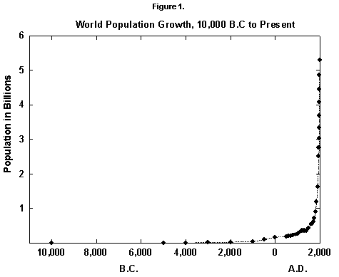
Fig. 1. World population growth, 10,000 B.C. to present. Sources of data: McEvedy and Jones [2] and United Nations [25].
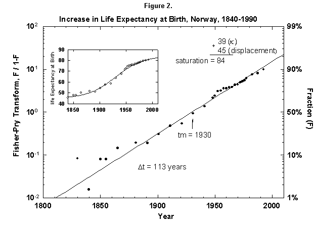
Fig. 2. Increase in life expectancy at birth, Norway, 1840-1990. A logistic curve fits the increase in life expectancy at birth. The logistic curve is displaced by 45 years, the life expectancy in 1845. As in most figures in this article, the logistic curve is plotted in both the traditional S-shaped form and in the Fisher-Pry transform. See Appendixes I and 2 for a description of the three parameters of the logistic model. Sources of data: United Nations [24] and Flora [16].
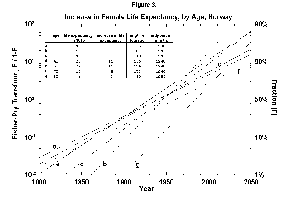
Fig. 3. Increase in female life expectancy, by age, Norway, 1800-2050. Logistic curves fit the increase in life expectancy at various ages. For example, an 80-year-old person could be expected to live 6 more years in 1815 and 9 more years in 1975, an increase of life expectancy of 3 years. A logistic is fit to the points between 1815 and 1975. Source of data: Flora [16].
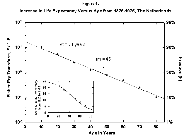
Fig. 4. Increase in life expectancy versus age, The Netherlands, 1825-1975. The figure shows that the increase In life expectancy is greater for the young than for the old, which implies an age limit. For example, a 10-year-old in 1975 had a life expectancy 24 years greater then in 1815. The actual life expectancy at each age is not shown on this graph. Source of data: Flora [16].
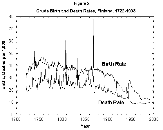
Fig. 5. Crude birth and death rates, Finland, 1722-1993. Birth and death rates have fallen by a factor of 4 since the 18th century. The fluctuations from the mean also have decreased drastically. Sources of data: Lutz [17] and United Nations [24].
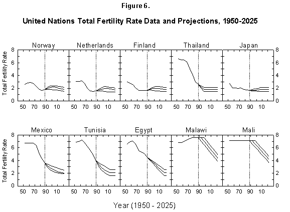
Fig. 6. United Nations total fertility rate data and projections, 1950-2025. The United Nations provides data and projections for 187 countries from 1950 to 2025. Source of data: United Nations [24].
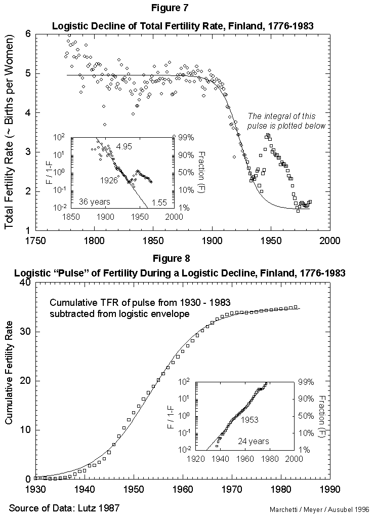
Fig. 7. Logistic decline of total fertility rate, Finland, 1776-1983. This figure fits a logistic curve to the decline in total fertility from a stable value in 1776 of 4.95 births per woman to the current value of 1.55 births per woman. The pulse of fertility in the 1940s and 1950s (squares) is modeled in Figure 8. Source of data: Lutz [17].
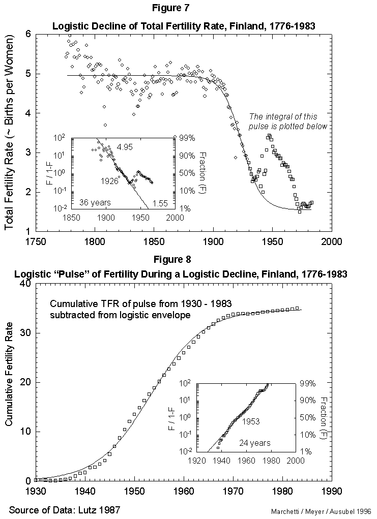
Fig. 8. Logistic “pulse” of fertility during a logistic decline, Finland, 1930-1983. This figure integrates the “pulse” of fertility evident in Figure 7 (the portion of the data plotted with squares instead of circles). The tbeoretical declining logistic curve was subtracted from this “bell-shaped” portion of the data, and the integral (cumulative sum) was then plotted and fit to a logistic curve to show the shape of the “babyboom” process. Source of data: Lutz [17].
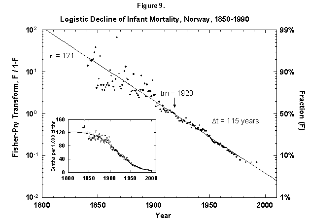
Fig. 9. Logistic decline of infant mortality, Norway, 1850-1990. The decline from 121 deaths per 1,000 infants born to 10 infants is dramatic and remarkably regular. The logistic was fit assuming a final goal of zero deaths, where the theoretical limit might be around 3 to 4, depending on advances in medical technology and screening procedures. Sources of data: Flora [46] and United Nations [24].
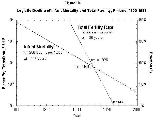
Fig. 10. Logistic declines of infant mortality and total fertility rate, Finland, 1800-1983. The Fisher-Pry transforms of the fitted logistics are plotted together for comparison. The data are not shown so as to ease comparison. Source of data: Lutz [17].
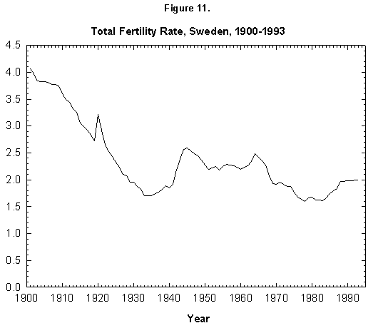
Fig. 11. Total fertility rate, Sweden, 1900-1993. Sources of data: Conseil de l’Europe [15] and United Nations [24].
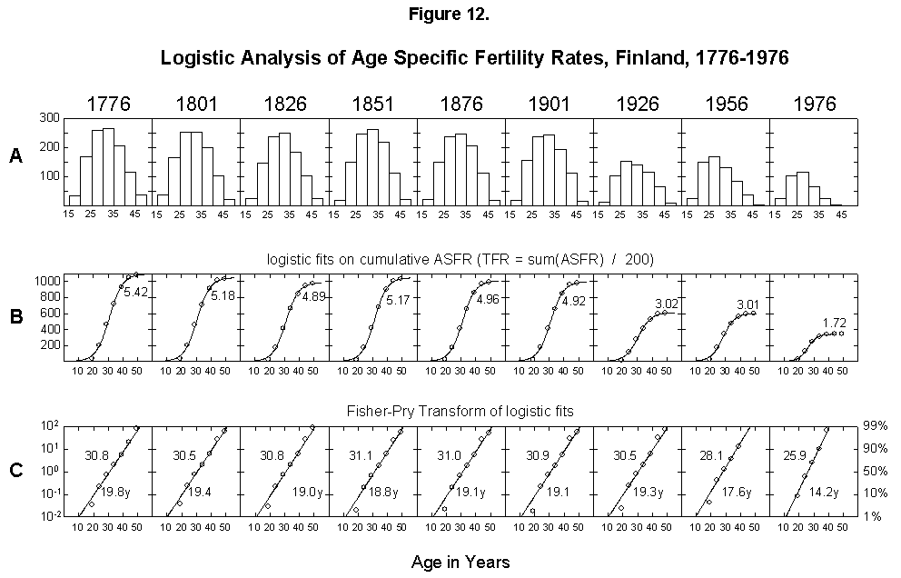
Fig. 12. Logistic analysis of age-specific fertility rates, Finland, 1776-1976. (A) Histograms of the age-specific fertility rates in 25-year intervals. (B) Integral (cumulative sum) of the bell-shaped histogram data, resulting in an S-shaped curve that is fitted with the three-parameter logistic. As explained in Appendix 3, the cumulative sum of the ASFR divided by 200 is equal to the total fertility rate (TFR). (C) Fisher-Pry transforms of the corresponding logistics (rendering them linear). Source of data: Lutz [17].
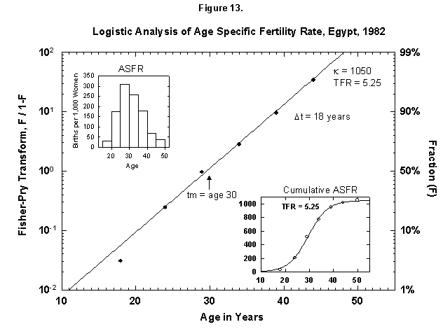
Fig. 13. Logistic analysis of age-specific fertility rates, Egypt, 1982. See Figure 12 and Appendix 3 for a description of the method of analysis used here. Source of data: United Nations [23].
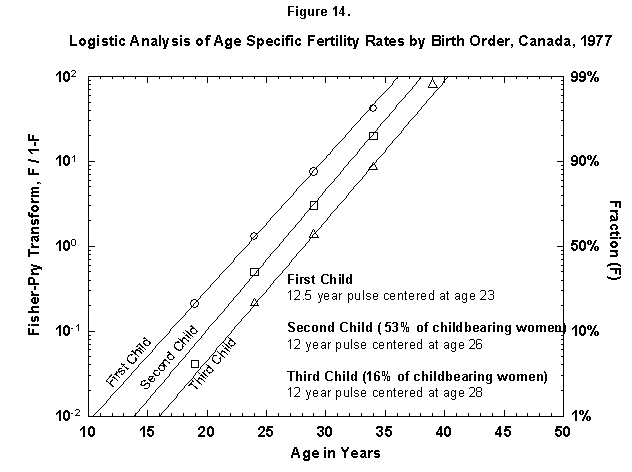
Fig. 14. Logistic analysis of age-specific fertility rates by birth order, Canada, 1977. The method of analysis used in this figure is similar to that used in Figure 12 and explained in Appendix 3, but here the fertility data are broken down further by the birth order, that is, first child, second child, and so on. The percentages refer to the number of women who go on to have more children (53% of Canadian childbearing women had a second child, but only 16% had a third child.) Source of data: United Nations [23].
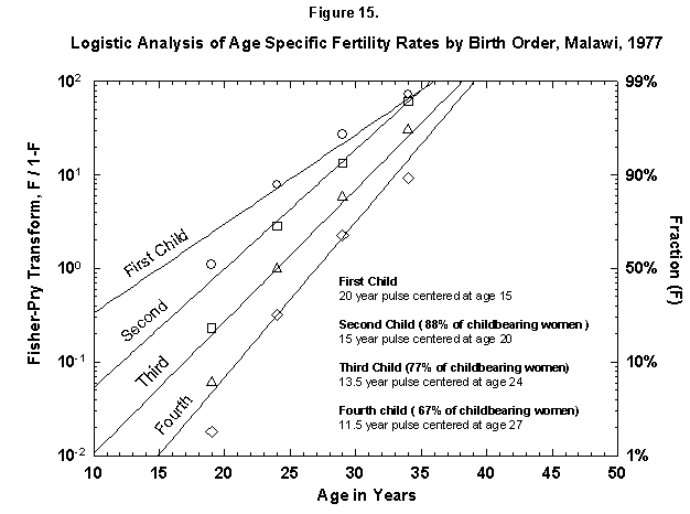
Fig. 15. Logistic analysis of age-specific fertility rates by birth order, Malawi, 1977. See Figure 14. Source of data: United Nations [23].
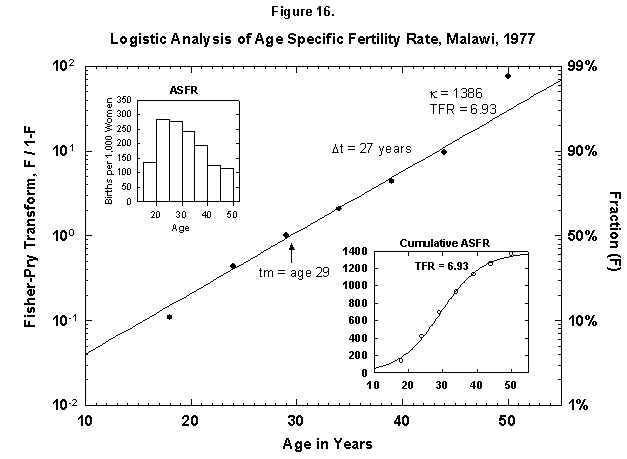
Fig. 16. Logistic analysis of age-specific fertility rates, Malawi, 1977. See Figure 12 and Appendix 3 for a description of the method of analysis used. Source of data: United Nations [23].
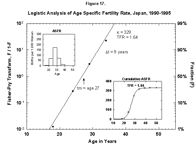
Fig. 17. Logistic analysis of age-specific fertility rates, Japan, 1990-95. See Figure 12 and Appendix 3 for a description of the method of analysis used. Source of data: United Nations [24].
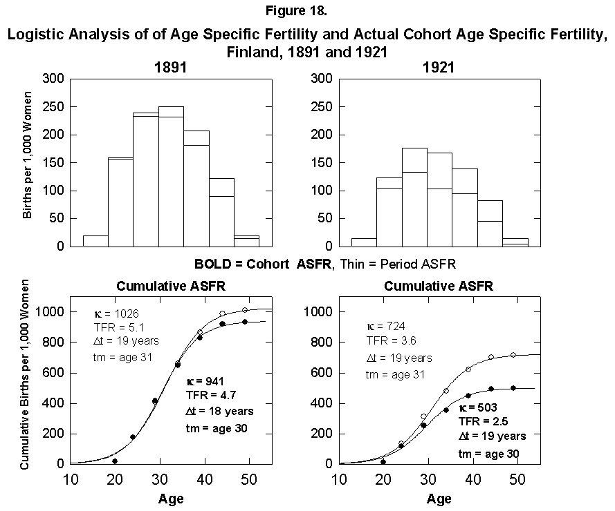
Fig. 18. Logistic analysis of age-specific fertility and actual cohort age-specific fertility, Finland, 1891 and 1921. Top: Histograms of both the ASFR and the Period ASFR, which follows the fertility rates of a 5-year cohort of women throughout their actual reproductive careers. Bottom: Corresponding logistics. PeriodASFR differ from the cohort ASFR when the fertility rates are rapidly changing, as shown by the 5-year age cohort from 1921 to 1961. Source of data: Lutz [17].
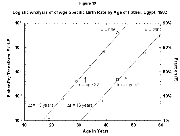
Fig. 19. Logistic analysis of age-specific birth rates by age of father, Egypt, 1982. This figure is similar to Figures 12-18 in that the cumulative ASFR is analyzed with logistics. However, this figure shows the cumulative ASFR by the age of the father as the sum of two logistic pulses. Source of data: United Nations [23].
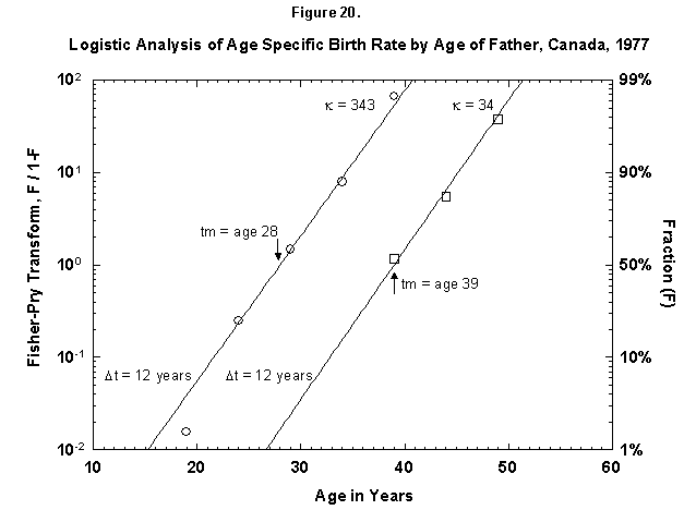
Fig. 20. Logistic analysis of age-specific birth rates by age of father, Canada, 1977. This figure shows the cumulative ASFR by the age of the father as the sum of two logistic pulses. Source of data: United Nations [23].
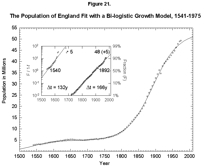
Fig. 21. The population of England fit with a bilogistic growth curve, 1541-1975. The sum of two logistics is used to analyze the population history of England. The first logistic curve has a 132-year characteristic growth time and a limit of 5 million and is centered in 1540. The second has a characteristic growth time of 166 years and a limit of 48 million and is centered in 1892. See Meyer [46] for a description of the bilogistic model. Sources of data: Wrigley [28] and Flora [46].
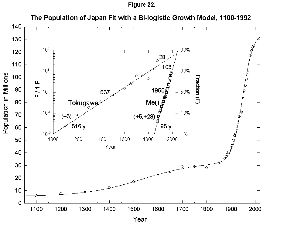
Fig. 22. The population of Japan fit with a bilogistic growth curve, 1100-1992. The sum of two logistics is used to analyze the population history of Japan. Adding on to an earlier base population of 5 million is a logistic with a 516-year characteristic growth time and a limit of 28 million centered in 1537. A second logistic curve with a 95-year characteristic growth time and a limit of 103 million centered in 1950 is added. See Meyer [46] for a description of the bilogistic model. Sources of data: Taeuber [21] and Tsuneta Yano Memorial Society [22].
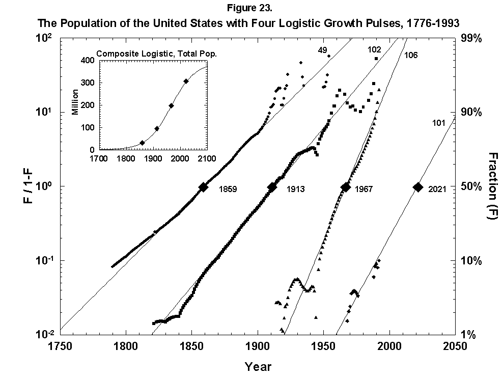
Fig. 23. The population of the United States with four logistic growth pulses, 1776-1993. The population of the United States is analyzed with the sum of four logistics centered on periods of rapid economic growth. The actual population is the sum of the logistics. In the inset the actual U.S. population data are fitted to a composite, or “superlogistic,” determined by the midpoints of the four component logistics. Sources of data: U.S. Bureau of the Census [26, 27].
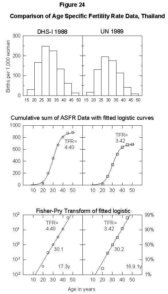
Appendix Fig. 1. Comparison of age-specific fertility rate data, Thailand. Left: Data from the Demographic and Health Survey (DHS). Right: UN data reported for the same year. Sources of data: United Nations [25] and Muhuri et al. [19].
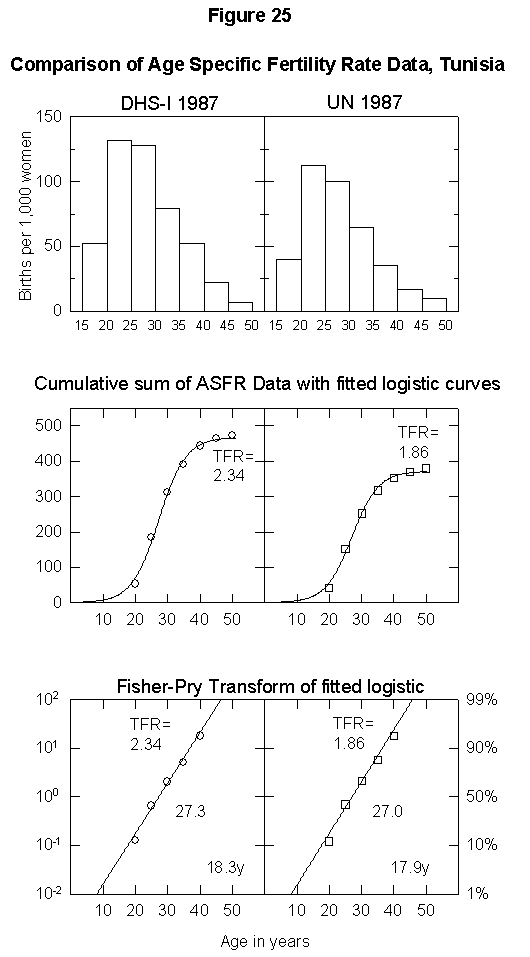
Appendix Fig. 2. Comparison of age-specific fertility rate data, Tunisia. Left: Data from the Demographic and Health Survey (DHS). Right: UN data reported for the same year. Sources of data: United Nations [25] and Muhuri et al. [19].References
I. Darwin, C., On the Origin of Species by Means of Natural Selection of the Preservation of Favoured Races in the Struggle for Life [1859], reprinted by Random House, New York, 1993.
2. McEvedy, C., and Jones, R., Atlas of World Population History, Penguin, New York, 1985.
3. von Foerster, H, Mora, M. P., and Amiot, L. W., Doomsday: Friday, 13 November, A.D. 2026, Science 132, 1291-1295 (1960).
4. Petersen, W., Population, 2nd ea., Macmillan, London, 1969, p. 333.
5. Keyfitz, N., Population: Facts and Methods of Demography, Freeman, San Francisco, 1971.
6. Keyfitz, N., Can Theory Improve Population Forecasts?, Report WP-82-39, IIASA, Laxenburg, Austria, May 1982.
7. Lutz, W., The Future Population of The World: What Can We Assume Today?, Earthscan Press, London, 1994.
8. Cohen, 1. E., How Many People Can the Earth Support?, Norton, New York, 1995.
9. Lee, R. D., and Tuljapurkar, S., Stochastic Population Forecasts for the United States: Beyond High, Medium, and Low, Journal of the American Statistical Association 89(428), 1175-1189 (1994).
10. United Nations, United Nations Demographic Yearbook, United Nations, New York, 1952.
11. United Nations, Long-Range World Population Projections: Two Centuries of Population Growth, 1950-2150, United Nations, New York, 1992.
12. Banks, R. B., Growth and Diffusion Phenomena: Mathematical Frameworks and Applications, Springer, Berlin, 1994.
13. Gruebler, A., and Nakicenovic, N., eds., Diffusion of Technologies and Social Behavior, Springer, Berlin, 1991.
14. Lotka, A. J., Elements of Physical Biology, Williams & Wilkins, Baltimore MD, 1924. Reprinted by Dover, New York, 1956.
15. Conseil de l’Europe, “La Fécondité des cohortes dans les états membres du conseil de l`Europe,” Etudes Démographiques 21, Strasbourg, 1990.
16. Flora, P., State, Economy, and Society in Western Europe, 1815-1975, St. James Press, Chicago, 1983.
17. Lutz, W., “Finnish Fertility Since 1722: Lessons from an Extended Decline,” The Population Research Institute at the Finnish Population and Family Welfare Federation, Helsinki, Finland, 1987.
18. Mitchell, B. R., European Historical Statistics, 1750-1975, 2nd rev. ea., Facts on File Publications, New York, 1981.
19. Muhuri, P. K., Blank, A. K., and Rutstein, S. O., Socioeconomic Differentials in Fertility, Demographic and Health Surveys Comparative Studies No. 13, Institute for Resource Development/Macro Systems, Inc., Columbia, MD, 1994.
20. Pressat, R., The Dictionary of Demography, Blackwell, Oxford, England, 1985.
21. Taeuber, 1. B., The Population History of Japan, Princeton University Press, Princeton, NJ, 1958.
22. Tsuneta Yano Memorial Society, NIPPON, A Charted Survey of Japan, Kokusei-Sha Corp., Tokyo, Japan, various years.
23. United Nations, 1986 Demographic Yearbook (Special Topic: Natality Statistics), United Nations, NewYork, 1988.
24. United Nations, World Population Prospects: The 1992 Revision, United Nations, New York, 1993.
25. United Nations, 1992 Demographic Yearbook (48th Issue Special Topic: Fertility and Mortality Statistics), Population Division, New York, 1994.
26. U.S. Bureau of the Census, Statistical Abstract of the United States: 1994(114 ed.), United States Department of Commerce, Washington, DC, 1994.
27. U.S. Bureau of the Census, Historical Statistics of the United States: Colonial Times to 1970, United States Department of Commerce, Washington, DC, 1975.
28. Wrigley, E. A., and Schofield, R. S., The Population History of England, 1541-1871: A Reconstruction. Edward Arnold Ltd., London, 1981.
29. Marchetti, C., Society as a Learning System, Technological Forecasting and Social Change 18(3), 267-282 (1980).
30. Yashin, A. 1., and Iachine, 1., How Long Can Humans Live? Lower Bound for Biological Limit of Human Longevity Calculated from Danish Twin Data Using Correlated Frailty Model, Mechanisms of Ageing and Development 80, 147-169 (1995).
31. Eigen, M., Self-Organization of Matter and the Evaluation of Biological Macromolecules, Die Naturwissenschaften 10, 465ff (1971).
32. Hausfater, C., and Hrdy, S., eds., Infanticide: Comparative and Evolutionary Perspectives, Aldine, New York, 1984.
33. Hirschman, C., Why Fertility Changes, Annual Review of Sociology 20 203-233 (1994).
34. Galloway, P. R., Basic Patterns in Annual Variation in Fertility, Nuptiality, Mortality, and Prices in Pre-industrial Europe, Population Studies 42, 275-302 (1988).
35. T. W, and Population Reference Bureau Staff, World Population in Transition, Population Bulletin 41(2), Population Reference Bureau, Washington, DC, 1991.
36. Imhoff, A. E., Die gewonnen Jahre: Von der Zunahme unserer Lebenspanne seit dreihundert Jahren oder von der Notwendigkeit einer neuen Einstellung zu Leben und Sterben, C. H. Beck, Munich, 1981, p. 53.
37. Rose, L., Massacre of the Innocents: Infanticide in Great Britain, 1800-1939, Routledge & Kegan Paul London, 1986.
38. Harris, M., and Ross, E. B., Death, Sex, and Fertility: Population Regulation in Preindustrial and Developing Societies, New York, Columbia University Press, 1987.
39. Ahn, N., Measuring the Value of Children by Sex and Age Using a Dynamic Programming Model, Review of Economic Studies 62, 361-379 (1995).
40. Riddle, J. M., Contraception and Abortion from the Ancient World to the Renaissance, Cambridge University Press, Harvard, 1992.
41. Move to Stop Sex-Test Abortion, Nature 324, 202 (1986).
42. Dickemann, M., Female Infanticide, Reproduction Strategies, and Social Stratification: A Preliminary Model, m Evolutionary Biology and Human Social Behavior: An Anthropological Perspective, N. Chagnon and W. Irons, eds., Duxbury Press, North Scituate, MA, 1979 p. 328.
43. Keyfitz, N., How Secure Is Social Security?, Report WP-81-101, IIASA, Laxenburg, Austria, July 1981.
44. Le Play, M. F., La Réforme sociale en France, Henri Plon, Paris, 1864, chap. 2.
45. Marchetti, C., Action Curves and Clockwork Geniuses, in Windows on Creativity and Invention, J. G. Richardson, ea., Lomond, Mt. Airy, MD, 1988, pp. 25-38.

46. Meyer, P., Bi-Logistic Growth, Technological Forecasting and Social Change 47(1), 89-102 (1994).
47. Smith, D., and Keyfitz, N., eds., Mathematical Demography: Selected Papers, Springer, Berlin and New York, 1977, pp. 333-347.
48. Kingsland, S., The Refractory Model: The Logistic Curve and the History of Population Ecology, The Quarterly Review of Biology 57, 29-52 (1982).
49. Putnam, P. C., Energy in the Future, Van Nostrand, New York, 1953.
50. Meade, N., and Islam, T., Forecasting with Growth Curves: An Empirical Comparison, International Journal of Forecasting 11, 199-215 (1995).
Received August 23, 1995; revised January 15, 1996; accepted January 16, 1995