Visualization of the model

There are many ways to visualize logistic growth aside from simple plotting on a linear scale. It is possible to define a change of variables that normalizes a logistic curve and renders it as a straight line (see Figure 2). This view is known as the Fisher-Pry³ Transform:

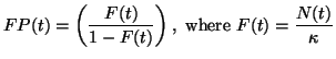$$FP(t) = \left( \frac{F(t)}{1 - F(t)}\right), \hbox{ where } F(t) = \frac{N(t)}{\kappa}$$ (3)

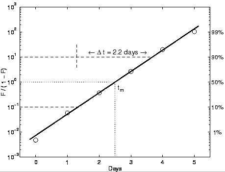
Figure 2: The logistic growth of a bacteria colony plotted using the Fisher-Pry transform that renders the logistic linear.

Note that

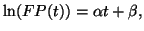$$\ln (FP(t)) = \alpha t + \beta,$$ (4)

so if $FP(t)$ is plotted on a logarithmic scale, the S-shaped logistic is rendered linear. We observe that the time in which the range is between $10^{-1}$ and $10^1$ is equal to $\Delta t$, and the time at $10^0$ is the point of inflection ($t_m$). Moreover, because the Fisher-Pry transform normalizes each curve to the carrying capacity $\kappa$, more than one logistic can be plotted on the same scale for comparison. As we will see, this becomes particularly useful when we analyze more complex growth behaviors. Figure 2 shows the Fisher-Pry transform of the bacteria example in figure 2. On the right axis we label the corresponding percent of saturation ( $100 * F$) at each order of magnitude from $10^-2$ to $1-^2$ rounded to the nearest percent.