Confidence Intervals on the Estimated Parameters: The Bootstrap

An important question to ask of a least-squares fit is ``How accurate are the estimated parameters for the data?''

In classical statistics, we are accustomed to have at our disposal not only single-valued estimates of a goodness of fit, but confidence intervals (C.I.) within which the true value is expected to lie. To ascertain the errors on the estimated parameters with classical statistics, the errors of the underlying data must be known. For example, if we know that the measurement errors for a particular dataset are normally distributed (far the most common assumption), with a known variance, we can estimate the error of the parameters.

However, for historical datasets, it is often impossible to know the distribution and variance of the errors in the data, and thus impossible to estimate the error in the fit. However, a relatively new statistical technique allows estimation of the errors in the parameters using a monte-carlo algorithm and the computational resources provided by modern PC's.

The Bootstrap Method [4] uses the residuals randomly picked from the least squares fit to generate synthetic datasets, which are then fit using the same least squares algorithm as used on the actual data. We synthesize, say, 1000 data sets and fit a curve to each set, giving us 1000 sets of parameters. By the Central Limit Theorem, we assume the sample mean of the bootstrapped parameter estimates are normally distributed. From these sets we can proceed to estimate confidence intervals for the parameters. From the confidence intervals of a parameter, we can form a confidence region which contains the set of all curves corresponding to all values of each parameter.

We first estimate the loglet parameters $\bold P$ using the least-squares algorithm described above and calculate the residuals $\bold R$ . We then create $n_{boot}$ synthetic datasets adding $R_{synth i}$ , a vector containing

residuals chosen at random (with replacement) from $\bold R$ :

$\displaystyle D_{synth i} = \bold N(t,\bold P) + \bold R_{synth i}$

The distribution of the parameters in $\bold P_{boot}$ is assumed to be normal, and thus the $95\%$ C.I. can be estimated by calculating the mean $\mu$ and standard deviation $\sigma$ of each parameter in $\bold P_{boot}$ , and using the formula:

$\displaystyle 95\%$ C.I. $\displaystyle : \mu \pm 1.96 \sigma$

Figure 8 shows a Bootstrap analysis of the Growth of a Sunflower (a ``classic'' logistic fit, available in the Loglet Lab gallery). Panel 8A shows the sunflower data fitted with a single logistic, with the parameter values estimated using the least-squares algorithm, $\Delta t = 50$ , $\kappa = 261$ , and

. Panels 8B, C, and D show histograms of the distributions of each parameter as determined by 1000 runs of the Bootstrap algorithm described above, along with the mean and $95\%$ C.I. marked by the solid lines.

**Figure 8:** 95% Confidence Intervals on the Estimated Parameters for the Growth of a Sunflower. The left side (A-D) shows the C.I. for all of the data, the right side (E-F) shows the C.I. obtained by masking the last five data points. Data from Thornton[19].
$\resizebox{4in}{!}{\includegraphics{suncomp.eps}}$

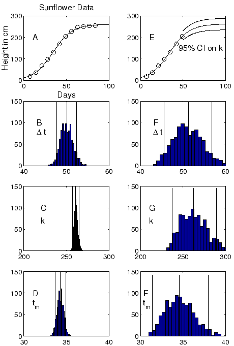To show how the completeness of a dataset influences the confidence interval, Panel 8E fits a single logistic to the same data, but now with the last five data points masked. The upper and lower solid lines show the $95\%$ C.I. on the value of $\kappa$ . Panels 8F, G, and H show the histograms and $95\%$ C.I. Notice that the C.I.'s have widened. Because the fit is now on a dataset that has not reached saturation, the prediction of the eventual saturation $\kappa$ is more chancey.

When performing a Bootstrap analysis in Loglet Lab, keep in mind the importance of first examining the residuals for outliers or other suspect data points. Reasons may exist to mask these outliers before performing the bootstrap, as a large residual value can unduly leverage a least-squares fitting algorithm. If the data are very noisy or contain many outliers, the least-squares algorithm might not converge during one of the many Bootstrap runs, producing unrealistic C.I.

The Loglet Lab software package performs the Bootstrap at the click of an icon. Use the same initial guesses for the Bootstrap as in the initial fit, so that the initial parameters values used in creating the synthetic datasets are the same. Each time the Bootstrap runs, a new seed is used for the random number generator used to pick the synthetic datasets, and thus each bootstrap analysis differs. For important analyses, performing the bootstrap a few times is wise. If the results are similar, high confidence can be placed on the the confidence intervals. For testing or debugging, it is possible to provide the seed manually, thus ensuring creation of the same synthetic dataset.