French Mobility: an example

This example illustrates logistic analysis of a data set with several components and masking. Figure 7 presents the results of an analysis of historical time-series data of French motorized mobility⁴. Periods of conflict, such as World War I, cause substantial deviations from normal activity; analysis of such trends, then, should focus on the years outside of these periods. That said, for this analysis, we excluded the data between 1912 and 1950.

We posit a logistic for the years of the Industrial Revolution, one for the advances in automotive production (i.e., the assembly line), and another for the post-WWII economic boom.

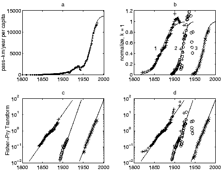
Figure 7a shows the data set $D$ (circles) and the estimated fitted curve $\bold N(t, \bold P)$, where

$$\bold P = \left[ \begin{array}{ccc} 53 & 322 & 1870 \\ 26 & 1291 & 1918 \\ 29 & 12254 & 1970 \end{array}\right].$$

Figure 7: Analysis of French Motorized Mobility

Accordingly, the weights $\bold w$ for the corresponding data points were set to 0.

Figure 7b shows the component logistics normalized to their respective $\kappa_i$ (for scale). Figure 7c shows the Fisher-Pry transform of the masked data set, while figure 7d shows the Fisher-Pry transform of all of the (unmasked) data.