Suppose we have ![]() technologies competing in a market over the course
of
technologies competing in a market over the course
of ![]() years. Our data representation now becomes a set of
years. Our data representation now becomes a set of ![]() vectors
of length
vectors
of length ![]() , or an
, or an
![]() matrix. To proceed with the model,
the first step is to transform the raw data,
matrix. To proceed with the model,
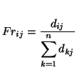
the first step is to transform the raw data, ![]() , into fractional
shares
, into fractional
shares ![]() of the market:
of the market:
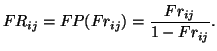
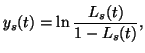
Secondly, the fractional shares ![]() are transformed using the
previously described Fisher-Pry transform
are transformed using the
previously described Fisher-Pry transform
The logistic substitution model generates substitution curves,
![]() , that correspond to the fractional market share data
, that correspond to the fractional market share data
![]() . The smooth curves follow the market share
through the three substitution phases: logistic growth, non-logistic
saturation, and logistic decline.
. The smooth curves follow the market share
through the three substitution phases: logistic growth, non-logistic
saturation, and logistic decline.
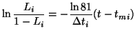
The first step in generating these curves from the logistic substitution model is to fit a curve to the growth phase of each technology. (Alternatively, as when data for the growth phase is unavailable for a particular technology, we fit a curve to its decline phase.) Reiterating from above, because we are working in the Fisher-Pry transform space, then
Note that for the logistic substitution model, we use a logistic with
only two parameters, because the third parameter, saturation level,
![]() , has fixed at 1, or 100%. Without the introduction of a new
technology, the last technology in the growth phase would grow to a
100% market share. If a new technology is introduced, its growth
must come at the cost (primarily) of the leading technology, causing
it it to saturate and decline.
, has fixed at 1, or 100%. Without the introduction of a new
technology, the last technology in the growth phase would grow to a
100% market share. If a new technology is introduced, its growth
must come at the cost (primarily) of the leading technology, causing
it it to saturate and decline.
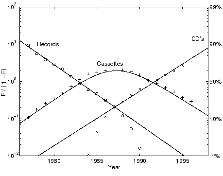
For each technology, it is necessary to specify the time window that represents its logistic growth (or decline). Within this time window are the data that will be used to estimate the parameters for the logistic that we just described. Figure 10 shows the logistic substitution model for the recording media data. The years 1975 to 1985 were used to estimate the logistic decline phase of LP's. The years 1977 to 1985 were used to model the logistic growth phase of cassettes. The years 1988 to 1996 were used to estimate the parameters for the logistic growth phase of CD's.
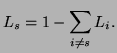
The growth and decline phases can be represented by logistic curves,
but this is not the case for the saturation phase. Because only one
technology, ![]() , can be saturating at a time, its market share can
be calculated by subtracting the sum of the shares of all the other
technologies-which must be known, since they must be either growing
or declining-from unity (100%):
, can be saturating at a time, its market share can
be calculated by subtracting the sum of the shares of all the other
technologies-which must be known, since they must be either growing
or declining-from unity (100%):
How do we know when each phase begins or ends? If
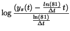 |
Figure 10 shows the logistic substitution model for U.S. recording media. In this example, the LP's are in the logistic decline phase, cassettes are in transition, and CD's are in logistic growth.