Next: Growth rates and the
Up: The Mathematics of Loglet
Previous: Definitions and notation
Contents
Now consider the set of  logistic components
 ,
where
,
where
where  is an arbitrary subspace of
  . (The components
  are analogous to
  as discussed in equation
(7).) A typical choice for is the interval
over which grows from 10% to 90% of its saturation level,
namely
as discussed in equation
(7).) A typical choice for is the interval
over which grows from 10% to 90% of its saturation level,
namely
 .
.
Restricting the domain of gives us a criterion for
decomposing the associated data set  into subsets
  (
(
 ) corresponding to each component logistic . A subset
contains a point
) corresponding to each component logistic . A subset
contains a point  if
if
 :
:
where  is the adjusted value of
  . The adjustment
is subtracting out the ``effects'' from other components,
leaving us with the (approximate) contribution of component to this
data point. In other words,
In Figure 5C, the hypothetical data set plotted in Figure
5A is decomposed into subsets
. The adjustment
is subtracting out the ``effects'' from other components,
leaving us with the (approximate) contribution of component to this
data point. In other words,
In Figure 5C, the hypothetical data set plotted in Figure
5A is decomposed into subsets  (circles) and
 (crosses); similarly, the fitted curve is also decomposed into
its component logistics. Note that the subsets are not
necessarily mutually exclusive in the domain; in this example,
and share points with common -values around
(crosses); similarly, the fitted curve is also decomposed into
its component logistics. Note that the subsets are not
necessarily mutually exclusive in the domain; in this example,
and share points with common -values around  .
At these times, we can see that there are two concurrent growth
processes; in addition, we can also quantify how much of the growth
can be attributed to each process.
.
At these times, we can see that there are two concurrent growth
processes; in addition, we can also quantify how much of the growth
can be attributed to each process.
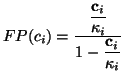
As we saw in Figure 3, we can apply the Fisher-Pry
transform to each component and its corresponding data subset. This
is useful because it normalizes each component on a semi-logarithmic
scale, allowing for easy comparison when plotted on the same graph.
Moreover, it allows the fitting of logistics using linear least
squares. The Fisher-Pry transform of components  is
is
where plotting  vs.
vs.
 produces
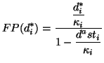
a straight line. The component data subsets are transformed in
a similar manner:
Figure 5D shows the
Fisher-Pry decomposition of the hypothetical data.
produces
a straight line. The component data subsets are transformed in
a similar manner:
Figure 5D shows the
Fisher-Pry decomposition of the hypothetical data.
Next: Growth rates and the
Up: The Mathematics of Loglet
Previous: Definitions and notation
Contents
Jason Yung
2004-01-28
![$\displaystyle d^\ast_i = d_i - \sum_{j \neq i} \frac{\bold P_{j2}}{1 +
\text{exp} \left[ {-\frac{\ln(81)}{\bold P_{j1}}}(t - \bold P_{j3}) \right] }
$](img67.png)