Human Population Dynamics Revisited with the Logistic Model: How Much Can Be Modeled and Predicted?

Citation: Technological Forecasting and Social Change 53: 1–30 1996

Keywords: Logistic curve model, population

Areas of Research: Diffusion of Social Phenomena

The following pages contain the full text and figures of an article which first appeared in the journal Technological Forecasting and Social Change, published by Elsevier Science Inc., New York, NY. Posted with permission.

Introduction: Runaway Growth or Slow Implosion?

As Charles Darwin said, in the struggle for life number gives the best insurance to win [1]. The Bible (Genesis 22:17) records that when God wanted to boost the elected ones, he promised that they would become more numerous than the grains of sand on the sea shore (i.e., >>10¹²).

In fact, world population since the mid 20th century has grown by about 2% per year, a rate that doubles the population in roughly 35 years. Actual data fitted over five centuries with reasonable equations show that the secular rate of growth kept increasing until around 1970, leading, at least from a mathematical point of view, to an infinite population in a finite time (Figure 1). (See [2] for a numerical history and [3] for an infinite prediction.) Such growth worries environmentalists and many others and leads to a first question: Where is the world population moving?

A second worry occupies rich, mostly white populations, in particular Europeans. The anxiety of their politicians and demographers (and the Pope) roots in the fact that on average a European woman now bears only about 1.4 children along her fertile span. To preserve a population, the rate should be around 2.1. The gap means that European populations are slowly imploding. An “oldies” boom preserves numbers for a while but empties society of the vis vitalis, the vital force carried by youth. Thus, a second question: Where is the population of the advanced industrialized nations moving?¹

Two mechanisms control the size of a population: life expectancy at various ages and the fertility rate. (Migration also affects the size of local populations, but we will not consider it here.) For both death and birth, demographers still are searching for working models, that is, numerical models corresponding to theory whose parameters are set by independent data and whose results pass the test of conforming to still other data. (See [5] for a classic introduction to demography; [6] for a severe critique of progress a decade later; and [7, 8] for the current state of affairs.) The absence of working models means that the demographers cannot forecast the evolution of either life expectancy or fertility. Lee and Tuljapurkar, for example, state: “Doubtless the most important source of error in population forecasts is uncertainty about future [fertility] rates, because these rates are changing over time in ways that so far have been difficult to predict or even to explain after the fact”[9]. Thus, population predictions are based on numerical assumptions, or guesses, or “scenarios.”²

So far, demographic predictions tend to diverge from the real numbers after about 20 years. To give some examples, in 1951 the Population Division of the United Nations (UN) estimated that the world population in 1980 [10] would be between 2.976 and 3.636 X 10⁹. The use of four significant figures for a scenario is certainly worth a note. The number in 1980 was actually 4.45 x 10⁹. In 1986 the UN predicted 6 x 10⁹ for the year 2000. The 1995 world population is 5.7 x 10⁹. The UN mark will probably be reached in 1997. The UN 1992 prediction for 2150 is a la carte [11]. One can choose seven different world population levels placed between 4.299 x 109 and 694.213 x 10⁹. However, the preference is for 11.543 x 10⁹. Unabated is the love for significant figures.

Predictions are always made with ifs. Because everybody seems scared by increasing human populations, fertility values are tamed in such a way-as to produce a maximum psychologically acceptable number of humans, usually between 10¹⁰ and 2 x 10¹⁰ by 2100. The reckoning date is well beyond the life expectancy of present politicians and demographers. These soothing predictions are obviously based on the if that current total fertility rates will fall everywhere to the conservation value of 2.1 (see Figure 6, later). As in weather forecasting, building the analysis from the bottom up becomes more and more complicated when one details to regions (and social status), and forecast results are not better.

Suffice it to say that the problem of the future size of humanity is unsolved. Whether the answer is unknown or unknowable, the problem partly lies in the methods, and no sign of breakthrough has appeared in the literature. Our response is to go back to the numbers and have a fresh look. We seek quantitative regularities to see whether it is possible to forecast with some internal logic where and when the growth will stop.

For both mortality and fertility all the mechanisms involved are regulatory and require social and cultural intervention. Because changes in culture and social behavior can be described by diffusive processes, basically captured in logistic equations (or their derivatives or sums), our fresh look will refuter the numbers along these lines. The fact that we can model with good precision over long periods several parameters usually looked at in charts in a qualitative way will show the strength of our method.

The use of the logistic model is widely established in many fields of modeling and forecasting [12, 13]. It has a controversial history in population ecology, a point to which we return near the end of this article. One of a family of density-dependent functions, the logistic law of growth assumes simply that systems grow exponentially under the constraints of an upper limit producing a typical S-shaped curve [14]. The three parameters of the logistic curve, which recur in our figures, are characteristic duration Dt, the limit K, and the midpoint t_m. The characteristic duration Dtis the time needed for the curve to grow from 10% to 90% of the limit K. Appendix 1 offers a mathematical description of the logistic model.

There is obvious need for demographic statistics of reasonable quality and consistent definitions. See [2, 11, 15-28] for data sources. We also offer precise definitions of terms in the Glossary, Appendix 2. Shortcomings arise in several ways. For example, although local demographic registrations are of ancient origin and reliable, their patching up into national statistics may not be. African states may have made written records only recently. Changing cultural values affect what is recorded. Years for which detailed survey data are available are few and do not include all countries. In Appendix 3 we give some quantitative examples of the uncertainty associated, even in the present day, with fertility rates. Nevertheless, we believe that the long-run and comparative nature of our approach makes the analyses robust.

Our plan is to look first from the bottom up, using the logistic to model life expectancy and then, in much greater detail, fertility. When cases are intractable analytically, as modeling human population has been, the alternative is to look from the top down with phenomenological insights. The master case is that of thermodynamics, where a couple of well-centered axioms permitted almost two centuries ago the construction of a branch of physics unchallenged to date. Its analytical counterpart, statistical mechanics, took a full century to develop. In the case of demography, analysis of the aggregate behavior or niche started for animal populations in the mid-1800s. Before concluding, we briefly reapply the logistic model to the analysis of aggregate human populations with the help of some extra hindsight.

Modeling Life Expectancy

Life expectancy is an important parameter in defining the size of a population because for a given birth rate the number of people is proportional to it.

Life expectancy in the developed world started changing in about 1800, improving slowly. The maximum gains have been in reducing infant mortality, but octogenarians also gained a few years. Demographers and medical doctors still struggle to define the future of the process. A simple solution can be found by assuming that each of us is endowed with longevity by DNA. Dangers along the way impede reaching the final age. However, by removing the dangers through nutrition, hygiene, medicine, and various coatings and protections, finally one can reach an age corresponding to longevity.

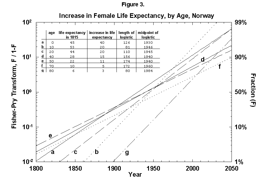
Because the removal of the dangers is a process of social learning, the equation most apt to describe it is a logistic [29]. For a time, knowledge and experience enable people to gain years of life with increasing speed. Then the process slows as we near the limits of efficacy of our various strategies. In fact, evolution of life expectancy during the last two centuries can be precisely mapped using logistics. In Norway the gain in life expectancy at birth forms a neat logistic taking off at the 1% level in 1810 and eventually adding 39 years to the life of the new-born Norwegian child (Figure 2). The process is logistic at each age, with 20-year-olds eventually gaining 20 years, 50-year-olds 11, and 80-year-olds 3 (Figure 3). In fact, one can also map with a logistic the final gain versus age, as we have done for the Dutch population (Figure 4).

All such analyses show that in developed countries we are near a limit [30]. Barring genetically engineered defense against senescence, life expectancy for women will stay in the mid-80s and for men about 5 years less.³ Consequently, the effect of increasing life expectancy on population, which for a while has masked the decrease in fertility in some rich countries, will disappear.

For developing countries we have not attempted to analyze comparable trends because the series of credible population statistics are not long enough. We would expect similar results. The basic processes of social development are the same, though perhaps operating more rapidly than they did for the countries that industrialized early. In developing countries, increase in life expectancy will sum up quickly, boosting the size of their populations on top of the effect of fertility.

In the long term, life expectancy acts as a fixed multiplier on population and is thus much less important than fertility, which acts exponentially.

Modeling fertility

Reproduction is at the center of life. As Manfred Eigen showed in his seminal papers 30 years ago, survival is the axiom from which the mathematics of life can be deduced [31]. But survival in an abrasive context means starting again and again, i.e., reproduction. Being central to survival, reproduction naturally also occupies a central place in the thinking and action of human societies. However, species are normally endowed with excessive reproductive capacity to take care of critical transients and occasional opportunities. Where survival rates are high, as in birds of prey who have few natural enemies, total fertility tends to be low. A chick every year or two for each female can suffice. Animals with lots of hungry enemies and poor defenses, such as snails, tend to astronomical prolificity.

These generic observations may have trickled down into the concept that in humans the transition to lower mortality will lead to a fertility transition to replacement levels. Visual observation of mortality and nasality curves for many nations shows in fact that both fall starting in the latter part of the 19th century (as shown for Finland in Figure 5). The reported decrease in mortality typically precedes that of fertility.

The post hoc propter hoc is necessary, but rarely sufficient, to determine a causal relationship. The two phenomena can descend from the same cause. To give a whimsical but not impossible mechanism, eating peanut butter could increase health and inhibit fertility. The phenomena could also be completely unrelated. A famous chart shows the decreasing number of storks flying to Germany during the last 30 years, closely matching the number of children born, by a constant multiplicative factor.

Certainly decreasing the mortality of infants and the young before reproductive age reduces the need to produce many offspring. But the human species is endowed with excess fertility that had to be, and was, pruned even before the decrease in mortality that came after 1800, to fix a round reference date.

A free-wheeling human female can produce a dozen or more children during her fertile period. Although this number was fairly frequently reached in agricultural families up to 1900, most families stopped at much lower levels, say 4 children born. This essential fact means that fertility was always under control, helped in case of necessity by infanticide, a practice widely used up to our days [32]. In Western countries infanticide is mostly substituted by abortion, which is the same act at a different time. Because fertility has always been under control, we must ask then why people stop at one number instead of another and, whether the choice, probably made without explicit reasoning, can nevertheless be rationalized.

Some years ago a striking attempt at rationalization was made for India. It was observed that India had a mortality transition, but did not seem to have a marked fertility transition. The mean number of children per family hovers around four. The rationale was that females in India usually do not hold stable paid jobs. The male provides cash for the family. Simple calculation shows that to have at any time at least one male in earning age, the family must shoot for two sons, that is, four children in the mean.

In a system where mechanisms external to the family do not provide old-age benefits, children are the only insurance for old age. Clearly, and the fact usually is not stressed enough, mechanisms for social security can be internal or external to the family but require children in both cases. With external mechanisms, as in the welfare state, the children in the system become a “common.” As extensively analyzed by socioecologists, this commons can suffer a tragedy if everyone takes away and nobody restores the resources. In fact, Western countries currently do not have enough children for ensuring the pension system, a point to which we return.

In short, the fertility situation is very confused, much more than transpires from the short considerations just outlined, and up to now fertility has escaped all model descriptions [33, 34]. Demographic books continue to be littered with puzzling charts and lists of numbers [35]. The UN projections of fertility express hopes for the future but no consistent view of mechanisms or continuity with the past (Figure 6). However, encouraged by our success in describing the evolution of life expectancy during the last two centuries, we believe that our logistic model deserves a chance.

Concerning the strategy of attack, the guidelines are simple:

1. Concentrate on age-specific fertility rates (number of children produced by 1,000 women of a given age cohort) to avoid the complexities of age structure in a given population and on total fertility rates (the average number of children per woman per lifetime).⁴
2. Spread the fertility rate analysis over countries of different cultural background and economic status.
3. Also look at the male side of the problem. Fertility rates are usually seen from the side of the female, but sometimes statistics also are available on birth rates according to age of the father.
4. Look at the hierarchical position of children according to birth order in different contexts in time and culture. Most women in Europe (and Japan) have only one child. The concerns about population stability move in opposite directions depending on the probability of multiple births.
5. Model the fertility transition per se, that is, phenomenologically, without theoretical (and emotional) constraints. Theory should adapt to facts.
6. Keep an eye on social moods. Because making children is deep, it will inevitably be moody. (The annual birth peak in late winter, reflecting increased conception in the spring and early summer, shows mood [36].)

As a reference case, we fit first the fertility data for Finland, a country with unusually good long records. Figure 7 reports the results for the time course of the total fertility (average number of children per female per lifetime). That course appears well approximated by a standard three-parameter logistic inserted between an early, rugged high plateau and a current low one. The year 1926 marks the midpoint of the logistic transition. Finland moved from a fertility rate of 4.95 in 1890 (99% of the upper limit) to a rate of 1.55 in 1962 (1% above the lower limit). The characteristic duration is 36 years.

On this secular evolution of total fertility rate, we find superposed a short pulse of extra fertility, as appears in Figure 7. Colloquially, it looks like the outcrop of the “baby boom.” This transient we analyze separately, integrating it in time. It also reduces to a logistic. The pulse centers in 1953, as seen in Figure 8. With the “baby boom” perturbation, we have described completely 200 years of total fertility in Finland. The model seems to work.

Now let us start our digging into the inner logic of fertility with a relation taken as extremely important as a causative agent in the present reduction of fertility in Western countries: fertility versus mortality. Many convoluted discussions exist on how and why one lags the other in the “demographic transition” from high to low death and birth rates.

Comparing the evolution of fertility with that of mortality requires some reflections. Mortality is usually fairly selective, hitting mostly children and old people. If we take total mortality, it mixes the two phenomena, which differ in psychological impact. We do not think reasonable a feedback process where female fertility is inhibited because octogenarians overcrowd the area. Certainly fertility in terms of population is diminished because of the dilution by infertile people. But, in terms of total fertility rates this dilution will not appear because the calculations refer to age cohorts of fertile females only.

In fact, our Finnish case also provides a comment on the possible mortality-fertility relation. As the “baby boom” fit appears good, we dare to backcast where the signals (good data) disappear in the noise of the recession and war years. In Figure 8 we then see that 1% of the phenomenon existed in 1929 (1953 minus 24 years). The situation for the world then was more bust than boom. It would be curious to explain the pulse as a compensation for the mortality of the war, if it began a decade before the war.

A narrower argument in the current literature is that when females see their children do not die, they make fewer. In 1800 in Europe one child out of four would die in the first years of life. Taking the reasoning ad litteram for Finland, compensation would occur in relation to a fertility in terms of survivors of 4.95 x 0.75 = 3.71. Total fertility in Finland in 1993 was 1.55, only 42% of the 3.71 we might now expect if this explanation sufficed. Certainly perceived values (e.g., of child survival) may differ from statistical ones, but other demographic examples show that people tend to perceive precisely, at least in the means.

Perhaps we can learn by looking at the secular evolution of infant mortality across cultures. Norway, analyzed logistically in Figure 9, shows that the model works again and that the reduction has a midpoint in 1920 and a characteristic duration of 115 years. France and Italy (not shown) have the same midpoint and characteristic durations of 88 and 110 years, respectively.

Returning to the Finnish case (Figure 10), when we compare the fitted logistics on fertility end infant mortality, we see similar midpoints, 1926 versus 1916, but very different root points (defined as 1% of the process), 1890 versus 1799. This temporal gap does not disprove a cause-and-effect mechanism, but it certainly weakens the argument. One must explain a delay of a century in setting up the process of reducing births.

Part of the explanation could be biased reporting. Clearly, fertility rate statistics can be falsified. Even in modern Europe, infanticide at birth was widely practiced, with no registration of the newborn if the decision had been taken to kill [37].

In our opinion, anthropologists Marvin Harris and Eric Ross [38] offer the key to the problem (see also [39] for an economist’s formalization). Looking at reproductive control in historical perspective, Harris and Ross show that people always had the tools. In other words, family planning always existed, as the decision to have or keep a child was taken inside the family. In the analysis of Harris and Ross, this planning tends to have an economic arrière pensée: are children a burden or an asset? Both, naturally. But the burden tends to fall on the female, and the asset accrues to the family as a whole.

In agricultural societies children are a clear plus. They become useful already about age 4. They run errands in place of adults, bringing food and messages to people working in the fields. They care for little stables, growing, for example, rabbits for the family. All at very little extra cost for the parents. The family systematically exploits youngsters until they marry and later if they remain in the patriarchal house. Old people run the system. They have, perhaps, the experience and, certainly, the authority to do so. The elders find in their command both social position and material support.

The patriarchal family was a welfare organization, perhaps more efficient and effective than the welfare state. A counterproof of this point of view is the presence of large families in proto-industrial English cities. In the words of Harris and Ross [38, 100], “A more plausible explanation for the early decline in mortality, which was most dramatic among infants, is that it was produced by a relaxation of infant mortality controls and by more careful nurturance in response to a new balance of child-rearing costs and benefits brought on by the shift to wage labor and industrial employment.”

With the expansion of factories, shops, mines, mills, transport, and other industrial capitalist enterprises, wage labor opportunities for children increased. Children became relatively more valuable, and infanticide, direct and indirect, yielded–though never entirely–to more positive nurturance.

This insight may resolve a paradox at the heart of demographic transition theory: that Europe experienced an explosive rise in population precisely at a time when, demographers have argued, Europeans were beginning consciously to control their fertility. What was new were the emergent material conditions, in particular, the magnitude of the incentive that industrial capitalism in the late 18^th and early 19th centuries presented for the alteration of behaviors that had heightened the risk of infant and child mortality.

This is not to say that the overall living standards of the multi-child family necessarily improved, but simply that wage-earner parents who reared more children were better off than those who reared fewer children under the existing conditions. Indeed, for the children themselves life was likely more “mean and brutish” than ever. Children were commonly fed at near starvation level until such time as it was necessary to fatten them up to go out and seek work. Descriptions in Victorian fiction abound. Charlotte Bronté’s Jane Eyre and Charles Dickens’ Nicholas Nickleby contain well-known examples.

The relaxation of infant mortality controls could manifest itself in the statistics. A diminution of direct and indirect infanticide is likely to show in demographic tables not only as a decrease in mortality but also as an increase in fertility. Live births previously regarded as spontaneous abortions or stillborn and never registered would, under a more nurturant behavioral regime, be registered as live births and distort the rate of fertility change in an upward direction. We have now reported Indian and European cases for pegging the “wanted children” number to a well-defined value. Harris and Ross [38] give examples since antiquity.

The “pill,” although scientifically made and certainly more reliable, did not introduce an essential discontinuity in birth control. Many types of contraceptives always existed in the form of vegetables and seeds that contained hormone mimics [40]. The Greeks and Romans, for example, extensively used a plant similar to fennel as an anticonceptional. The plant grew wild in Libya. To stress its commercial value, the Romans minted its image on coins, so that the plant can be exactly identified. Significantly, it was harvested to extinction.

Assuming that economic considerations prevail, let us now look at the present situation in developed countries. All of them are in a phase of low fertility. The current wisdom assumes that wealth is an opportunity for selfishness where personal pleasure is put before the toils of rearing children.

Historically, even in periods of high fertility, the wealthy have had few children. This argument often pops up, helped by the argument of feminist power and female careers. Clearly, in a well-off family children are not assets. They are costly to grow and educate at the appropriate standard. They bring no income when they are young. They are unnecessary for the support of their aging but still wealthy parents. If static property such as land forms the wealth, many children would inevitably split it. These trivial reasons neatly explain the premodern demographic practices of the rich. Fertility control has never been a real problem, although infanticide would have been more complicated in a wealthy environment.

Nowadays wealth at large is linked more to financial assets than to static property, but child costs still can be described the same way. Nurturing the oldies is left to third parties financed by the income or assets of the old people. In this situation of no economic incentive, only one basic reproductive instinct remains, that of continuity. Adults beyond reproductive age who realize that there is nothing after them rage and despair. Their genes will disappear. Metaphorically, the rocket went into space without a payload.

Assuming that the basic instinct for continuity is finally stronger than bare economic considerations, then every couple may long for a child. With the very low level of child mortality at present (around 1%), one child should be enough. But here another argument, or instinct, comes in. The child should be male. If we put biological mechanisms in control, this request makes sense, as otherwise the Y gene would be lost.

It is difficult to demonstrate that the cultural biases leading to the same conclusion are an externalization of the basic instinct under folkloric disguise. However, suppose couples reproduce starting with the idea of the boy. 50 percent of them, or a few more, get one. The other half get a girl and a dilemma: what to do next. We may assume that they decide on a second try. The last, if unsuccessful.

With this strategy in mind, and taking into account that about 15% of the females never give birth for various reasons, we find a reproduction rate of about 1.3 per female, almost exactly the present reproduction rate in European countries.⁵ If our reasoning is correct, their situation is unlikely to change, because of a lack of driving forces in the short term.

On the other hand, the potential exists for further decline, because modern techniques permit the determination of the sex of the fetus at an early age. Such potential is realized already, for example in India, where, as described, two males per family are in request. Ninety-nine percent of the abortions following sex determination in India are females. (One study of 8,000 cases of abortion in India showed 7997 female fetuses [41].) This excess female “mortality” has been a historically omnipresent phenomenon. In China l9th-century surveys report male-female childhood sex ratios up to 4 to 1 as late as the 1870s [42]. Prostitution obviously flourished, and concubines’ flagged status.

In Western countries, the economic detachment of parents from children may bring another scenario and perhaps set restoring forces into action. A population with a total reproductive rate of 1.3 per female is unstable and converges to very small numbers in a few generations. Children are decoupled from the family, but they are still coupled to society because, collectively, they must earn the pensions paid to old-timers.

As suggested, shrinking the total number of children will wreck the pension system, bringing a feedback signal already strong after two generations, well ahead of the shrinking to zero of the total population [43]. History shows such reasoning to be correct. We report one case in which the same social context, land, and population under different laws produce different, and predictable, results.

Before the French Revolution, primogeniture determined the inheritance of land. The eldest child inherited all. The 1789 revolution brought the abolition of the rights of the eldest child in 1790-1791. Equal partition followed under the Napoleonic code. Consequently, fertility shrank to the point of producing only one son per family. The loss of inheritance by splitting would mean a loss of liberty and downward social mobility. The only lever left to the family than was to reduce the number of offspring, and they used it. Pierre Le Play, the 19th-century developer of the social survey, observed that the Ancien Regime produced the eldest son, whereas the new produced the only son [44].

When opportunity knocks, the rich may also procreate profusely. Royal families provide a typical case. They use children to consolidate power by putting them into the administration and the army and to penetrate external territories via marriages. Empress Maria Theresia, a career woman with heavy duties had, nevertheless, 17 children. Her Habsburg family actively procreated for 1,000 years, perhaps one of the roots of its continuing power. They still appear now as a big bunch, and they might come back, as adumbrated by the recent proposal to Otto to become king of Hungary.

Conversely, civilizations have simply melted away because of poor reproductive rates of the dominant class. We should not forget that the white man’s supremacy started with a reproductive stir in Europe during the last part of the first millennium and continued with ups and downs until the end of the 19th century. The question may be whether underneath the personal decision to procreate lies a subliminal social mood influencing the process, as endorphins do. The fact that crude birth rates in Austria jumped up by 60% in 1939, the year after the German annexation, may not be pure chance. The subliminal mood of the Europeans could now be for a blackout after 1,000 years on stage.

Sweden counters the trend to the lowering (to 1.3) of the total fertility in Europe. Swedes, after a decrease from a value of 2.5 in 1964 to 1.6 in 1977, started a rise in 1983, bringing the value back to 2.0 in 1992 (Figure 11). Examining the phenomenology of this change by fine analysis of fertility pattern would be useful.

Logistic equations have successfully described the growth of an individual and the evolution of the vis vitalis in integral form, counting, for example, the publications of a scientist or the works of an artist [45]. Thus, it is natural, heuristically, to try them on fertility versus age. Children are a form of DNA publication, after all. Fertility statistics include reports of female fertility as a function of age, usually in blocks of 5 years. Fathers are not neglected; births according to the age of the father are sometimes available.

Figure 12 shows the result for Finland at intervals from 1776 to 1976. When we think of all the whimsical forces presiding over reproduction, the fitting appears excellent. The first datum is usually low with respect to the fitted curve, a general characteristic of the fitting of vis vitalis interpretable to mean that the young have the drive but not yet the tools (for the artist). In the case of young girls, society constrains. But, in short order, the lost activity is made up, and the second point is perfectly in line.

Our frugal condensation of the characteristics of fertility into a few numbers makes quantitative comparisons convenient. We can, for example, compare the fertility rates over time. Comparison shows that the reproductive activity concentrates in younger and younger years, the midpoints moving from 30 to 31 years old in 1776-1926 and to 26 in 1976. The characteristic duration of the process shortens from 20 years to 14. The time structure remains, as the profile of the histograms in Figure 12 basically stays the same. In accounting terms, clearly children of higher rank (n + 1) are falling off. The perfect self-consistency shows that the planning, if subliminal, precedes the accident (e.g., an abortion).

This analysis also makes comparison sharp for different cultures, and certainly the biological dictates are cross-cultural. In Egypt (Figure 13) a woman now produces the number of children more or less that a Finnish woman did 100 years ago. We find an analogous distribution in time, as the Egyptian midpoint is 30 years (as for Finland to the 1920s), and the characteristic duration is 18 years (vs. 19). One might think that the preset number of children determines the time pattern of pregnancies.

We can zoom into further detail, such as the distribution in time of deliveries according to the sequence of children (first, second, etc.), for example, for Canadian females (Figure 14). The time structure in the production of the first child is basically identical to that of the following ones. The distance between the child waves is about 2.5 years (the numbers for the midpoints are rounded). Such Prussian order was certainly unexpected in such amateurish activity. The probability for a third Canadian child falls off rapidly.

Very ordered, if not in a Prussian row, are also Malawi women (Figure 15), who seem to shoot in faster and faster flashes. Probabilities decrease very slowly for successive children, and so Malawi grows rapidly. Only the first four children are analyzed in Figure 15, but the total nears seven (Figure 16). The pattern may resemble that of Finland around 1700. The physical fertility span seems busy all over. The characteristic duration is longer for Malawi women.

Speaking of time constants, at the other extreme we find Japan, where the characteristic duration of the age-specific fertility rate is only 9 years, meaning that all the children are produced near the midpoint, 27 years (Figure 17). The number is only 1.6 per female.

These few examples, extracted from a large portfolio, do not show any special feature that characterizes female fertility in a way that permits the forecast of the fertility of a certain group. Obviously the fertile period expands or contracts to accommodate more or fewer children. The central point does not move much away from 28 years. The consistency of the process impresses, as if the decision to produce n children were taken before starting. Recall that the statistics are longitudinalized, that is, taken at a certain date for women of various age brackets. The integration assumes that data refer to a certain cohort (by date of birth) observed along its life span.

The total fertile period for women is about 35 years. For the few places where statistics are available, it is interesting to integrate for a given actual cohort across years of large fertility change to see whether the presumed family plan is kept across the change. We perform the experiment for Finnish women, for whom we know 1926 was the peak year of change in fertility rates. (Long time-series data on cohort fertility are also available for France and several other European countries [15].) We take cohorts born in the periods 1881-1885 and 1921-1925 with midpoints around 1914 and 1952. We need to keep in mind the reproductive doldrums circa 1930.

Figure 18 compares the cohort and period fertility rates in Finland and shows that the actual cohorts do experience the lower fertility into which they will grow. We might interpret this to indicate that the women in some way anticipate the future trend or that the trend of the time when they were around the center point had a dominant effect on their behavior, and the tails were somehow adjusted.

Let us check the symmetric case of male fertility. For animals, including humans, the female obviously makes the biological decision, but the male behavior might mirror the decisions in a revealing way. Figure 19 reports male fertility (age of father when a legitimate child is born) for Egypt. Here we see a curious phenomenon involving two logistics, or “bilogistic growth” [46]. A first wave of procreation, similar to that of a female, generates most children. Then a second wave follows, at a midpoint distance of about 15 years, as the aging father has a second pulse of procreation (midpoint 47 years) with about one-fourth of the children of the first. One might think that in predominantly Moslem Egypt, men, having attained with age a certain economic success, refresh their harems. But the same phenomenon also appears in Canada, a country of very mixed religion (Figure 20). The midpoint distance between the spurts is less than in Egypt, 11 years, and the size of the second spurt is only about one-tenth of the first. Divorce, common in countries such as Canada, permits longitudinal polygamy, and consequently the final result may be the same. Canadian men reach 90 percent of their second wave of fathering by 45, whereas Egyptian men take until 55.

In a nutshell, high fertility appears to be the effect of protracted fertility, both for male and female. Simple observation makes this conclusion fairly obvious, but here we report it in crisp mathematics that may help the next step in conceptualization. More generally, we have seen that many individual demographic processes are well modeled by the logistic. Although interesting per se, the analysis of fertility does not give clues for the future. For example, our historical analysis of Finnish women (Figure 7) shows the transient but carries no logic to foresee or negate a new transient either up or down. Notwithstanding the considerable success in the morphology of fertility, the assembly of the mechanisms that enable population forecasts from the bottom up has yet to come.

Modeling the Niche

Alternatively, forecasts of population may be made by methods that look at the aggregate numbers and neglect the mechanisms. After all, animal societies growing in a given niche have numerical dynamics neatly fitted by logistic equations with constant limit K. The idea originated in Europe in the middle of last century and reached its maximum splendor in the United States in the 1920s with the work of Pearl, Reed, and Lotka (reproduced in [47]; see also [48]). Putnam resumed this work after World War II [49]. His brilliant recapitulation remains worth attentive reading.

What these investigators found is that logistics usually fit well the growth of a human population for a while, but then often problems come. The mathematicians and statisticians who looked into the problems tried to solve them with the tool they were most familiar with: mathematics. They invented “generalized” logistics of various descriptions and increasing complication, until it was no longer worthwhile to do with these logistics what could be done with polynomials [12]. In any case, the capacity to predict eluded the analysts.

The reason why the logistics work well with most animal populations is that the niches that encase the populations are of constant size. When the animals can invent new technologies, such as when bacteria produce a new enzyme to dismantle a sleepy component of their broth, then we face a problem. New logistics suddenly pop up, either growing from the limit of the prior one or, if the invention came early, in the course of the first logistic.

This expansion of the niche happens with humans. In fact, homo faber keeps inventing all the time, so that logistics have fleeting limits. To give an example, if we take the “industrial revolution” as one very large innovation (embracing the changes discussed earlier in mortality and fertility), we can reconceive the population history of England as a sum of two logistics, or bilogistic, with the first limit set by medieval technology at 5 million and the second limit rising to accommodate 48 million more in the modern era [46] (Figure 21). Japan, which was largely impervious to Western technology under the Tokugawa Shogunate and then absorbed it eagerly under the Meiji beginning in the 1860s, provides an even cleaner example with an addition of 103 million to a base of 33 (Figure 22).

Abandoning restraint, we have also mapped the growth of the U.S. population with a sum of overlapping logistics keyed to long cycles of economic expansion (Figure 23). The fit is not bad, but equally good alternative fits exist, and interpretation is fuzzy. As with forecasting fertility, the method does not say what will come next. One trick we can try, which has worked post-mortem in other analyses, is to envelop the sum of logistics in a “superlogistic” constructed by taking as base points the centerpoints of the single logistics, loaded with the values of the respective limits. We bring the masses into the gravity centers, so to speak. The result for the United States, shown in the inset of Figure 23, is that the population grows to a limit of around 390 million roughly in 2100. The midpoint is around 1940 when the United States became world power #1. All the figures appear plausible, but the exercise is acrobatic.

On niche approaches, we might summarize by saying that so far no one has built a solid structure capable of propelling itself into the future. As the case of the growth of the population of the United States shows, just fitting equations provides no roots to keep the results standing. However, we cannot help but be impressed by the factors of increase between apparent population limits, 10 in England and 4 in Japan.

Conclusions

The revival of the logistic brings substantial progress in the modeling of the evolution of life expectancy and of fertility versus age. Life expectancy grows at all ages, with different rates, according to a logistic path. In looking at the limits of these logistics, when no more gain should be expected, we find convergent paths. Thus, mortality all along the life span will be reduced to small numbers and mortality concentrated toward the end. Death comes through senility, and the mean age of death, when the limit of our logistic life span occurs, can be defined as longevity. For Europeans (and probably everyone eventually), it is about 80 years for men and 85 for women.

The longevity “pill” could come with genetic engineering, but in any case we doubt it will be demographically important until after, say, 2050. Its diffusion will be limited by experimentation and investigation of its effects. Although life expectancy above 50 years of age greatly affects social organization, its change has only transitory effect on total population numbers.

Fertility dynamics also follow logistic paths. The retrospective analysis of fertility (and mortality) afforded by the logistic undermines several popular arguments in demographic theory. It supports the view that fertility has always been under cultural control and that family plans, beyond one son, are essentially economic. In the absence of fears about the future of social security or other conceptional stimuli (or massive immigration), the populations of the advanced industrialized nations will slowly implode. Admitting such “ifs,” we have not solved the problem of modeling total fertility in the future, on which prediction of the population as a whole depends.

However, the logistic can offer a consistent approach for predicting values for variables in demographic models, including those that take into account the changing age structure of a population, provided the logistic character of the process is reasonably established and no “new logistic” arises. These values are logically superior to the guesses now incorporated into many models.

With respect to niche approaches, logistic analysis at least formally and quantitatively defines the problem of limits. The growth of human populations demonstrates the elasticity of the human niche, determined largely by technology. For the homo faber, the limits to numbers keep shifting, in the English case by a factor of 10 in less than two centuries. In the long run, these moving edges probably most confound forecasting the size of humanity.

We are grateful to Thomas Buettner, Joel Cohen, and Paul Waggoner for assistance.

Appendix 1: The Logistic Model

This appendix defines the logistic model and the terms we use for demographic analysis. The logistic model assumes that the early growth of a population (or other variable) N(t) increases exponentially with a growth rate constant a. As the population N(t) approaches a limit k, the growth rate [dN(t)]/dt slows, producing the characteristic S-shaped curve. The mechanisms that cause this slowing depend on characteristics of the population or system being modeled, but empirical studies have shown that this slowing is present in many growth and diffusion processes. Thus, the logistic is a useful generic model for both systems where the mechanisms are understood and where the mechanisms might be hidden.

The continuous nonlinear ordinary differential equation that describes this growth process is:

For the analytic form we need a third parameter, t_m, which specifies the midpoint of the sigmoidal curve and is related to the initial population N_o(t) by

We also replace a with Dt, the characteristic duration, that is, the time it takes the population N(t) to grow from 10% to 90% of the limit k. Dt is related to a by Dt = In81/a. The analytic form of this differential equation, with our parameterization, is:

It also is possible to define a change of variables that allows a normalized logistic to be plotted as a straight line (often known as the Fisher-Pry Transform):

If FP is plotted on a logarithmic scale, the S-shaped logistic is rendered linear and the period between 10^-2 and 10² equals At. The FP transform also allows more than one logistic to be shown on the same graph with the same scale, as each curve is normalized to the limit k.

Literally thousands of examples of the dynamics of populations and other growth processes have been well modeled by the simple logistic. Classic examples include the cumulative growth of a child’s vocabulary and the adoption of hybrid corn by lowa farmers. The excellent fits obtained are a major reason for our preference for the logistic. Another advantage of our formulation of the model is that its parameters have clear, physical interpretations. In addition, recent studies have shown that the simple logistic often outperforms more complicated parameterizations, which have the disadvantage of losing clear physical interpretations for their parameters [50].

Appendix 2: Glossary of Terms

Fertility: The childbearing performance of individuals, couples, groups, or populations. General fertility rate (GFR): The ratio of the number of live births in a specified period (often I year) to the average number of women of childbearing age (usually taken as age 15-49) in the population during the period. For example, the U.S. GFR for 1990 was 31.8 births per 1,000 women age 15-49 per year [24].

Age-specific fertility rate (ASFR): The number of live births occurring to women of a particular age or age group per year, normally expressed per 1,000 women. For example, the ASFR for U.S. women age 20-24 was 122.1 births per 1,000 women in 1990 [24].

Total fertility rate (TFR): The TFR can be interpreted as the number of children a woman would have during her lifetime if she were to experience the fertility rates of the period at each age. The TFR is obtained by summing the age-specific fertility rates (ASFR) over the whole range of reproductive ages for a particular period (usually 1 year). Although one of the most frequently quoted measures of fertility, the TFR sometimes requires a certain caution in interpretation. It is a hypothetical measure, not necessarily applicable to any true cohort, and may be of dubious value when the level or timing of fertility are changing. A TFR of 2.1 is a widely cited benchmark for a stable population. The U.S. TFR for 1990 was 1.92 births per woman, the world average in 1990 was 3.45. Africa averaged the highest TFR in 1990 at 6.24 [24].

Cumulative age-specific fertility rate: This rate is equivalent to the total fertility rate. As stated in the definition for TFR, the TFR is the sum of the Age-specific fertility rates (ASFR) over the whole range of reproductive ages. An example will make this clearer. Egypt in 1982 had an ASFR distribution as shown in Appendix Table 1.

Because there are 5 years per age group, the sum of the ASFR values in the table (1,055.2) multiplied by 5 gives the TFR in births per 1,000 women (5,276 births per 1,000 woman per lifetime). It is customary to give the TFR in births per woman, in this case approximately 5.3 births per woman per lifetime. Thus, the Cumulative ASFR divided by 200 equals the TFR.

Notice that the distribution of the ASFR, when plotted as a histogram, approximates a bell-shaped curve. The cumulative sum of a bell-shaped curve is an S-shaped curve. Thus, we use the well known S-shaped logistic growth curve to characterize the cumulative ASFR of different countries. The three parameters of the logistic curve are characteristic duration Dt, limit – k, and midpoint – t_m. The characteristic duration Dt is the length of time needed for the curve to grow from 10% to 90% of the limit, which in this case roughly translates to the length of the childbearing process for a given ASFR distribution. The limit k is equivalent to the TFR, and the midpoint t_m, the center of the curve.

Age-specific fertility rate by birth order (ASFR): Very rarely, the ASFR of a population is broken down by birth order. For example, in Egypt in 1982, women age 20-24 had 173.9 births per 1,000 women. Of those births, 56.7/1,000 were from women having their first child, 68.0/1,000 were from women having their second child, and so on [23].

Crude birth rate: The ratio of live births in a specified period (usually 1 year) to the average population (normally mid-year population) in that period, usually in births per 1,000 persons. Varies from 10 per 1,000 in developed countries to 60 per 1,000 in the developing countries. The U.S. crude birth rate for 1990 was 16 per 1,000 persons [24].

Crude death rate: The ratio of deaths in a year to the population, usually given in deaths per 1,000 persons. The crude death rate (also called simply the death rate) is strongly influenced by the age-sex structure of a population. The lowest death rates are to be expected in rapidly growing or youthful populations with a high life expectancy. For example, Singapore in 1980 had a death rate of 5 per 1,000, whereas the U.S. death rate for 1980 was 8.6 per 1,000 [24]. In historical times, the crude death rate might have been as high as 30-40 per 1,000, with crises years reaching rates twice as high.

Mortality: The process whereby death occur in a population.

Infant mortality rate: The ratio of the number of deaths during a specific period (usually 1 year) of live-born infants who have not reached their first birthday to the number of live births in the period. It is usually given in deaths per 1,000 live births. The infant mortality rate for the United States in 1990 was 10 deaths per 1,000 live births [24].

Life expectancy: The average number of additional years a person would live if the mortality conditions used in the calculation remain valid. Usually given as life expectancy at birth, which can vary from 80 + years for females in the developed countries to 40 to 50 years in the developing countries. Sometimes given as life expectancy at age X, which gives the average additional number of years a person at age X can be expected to live.

Appendix 3: Note on the Problems with Fertility Data

A major obstacle to accurate demographic modeling is uncertainty in the available data, especially for the developing countries. In countries where births and deaths are not recorded, it is hard to construct accurate population estimates and even harder to reconstruct age-specific fertility rate (ASFR) data needed for accurate population modeling. For these countries, a few widely quoted publications contain data derived from different sources.

The United Nations Demographic Yearbooks contain data collected from the national statistics offices of the member countries. For countries with good national statistics agencies, the data are accurate, but for the others the data can be unreliable. For example, some countries’ statistics agencies might, for political or social reasons, underreport the data on various subpopulations. For this reason, the United Nations World Population Prospects projections do not rely exclusively on the data provided by the national statistics agencies, but supplement them with data from independent surveys conducted by academics, other national or international nongovernmental agencies, or the World Bank. Another source of data is the Demographic and Health Surveys (DHS) project run by the Institute for Resource Development, Inc., Columbia, Maryland. The main objective of this 9-year project is to “advance survey methodologies [in the developing countries] and to aid in the development of the skills necessary to conduct demographic and health surveys.” The data for the participating countries are considered reliable.

To illustrate the uncertainty in fertility data, Appendix Figure 1 and Appendix Figure 2 show comparisons between the ASFR data on Thailand and Tunisia from the United Nations Demographic Yearbook (national statistics) and the DHS surveys. In the case of Thailand, the estimated total fertility rate is either 2.34 births per woman or 1.85, the former being above and the latter below replacement level. The data for Tunisia also differ by one child per woman. Uncertainty of this magnitude could significantly bias population projections. Clearly, better data are necessary for accurate population modeling.

ENDNOTES

¹ Such fear dates back to the 1930s [4].

² For example, Lee and Tuljapurkar [9] assume that the U. S. fertility rate will converge to 2.1, the replacement level: “Conventional time series models for fertility can lead to unrealistic forecasts (including negative fertilities), so we examined two alternative models that incorporate prior information…. In both alternatives we constrain the models so that they yield a prescribed ultimate average value of the total fertility rate. We used a mean of 2.1, chosen in part because it is close to the ultimate level of the 1992 Census projection and in part because many demographers view such an assumption as appropriate.”

³ See also the following article in this issue by Marchetti for additional examples and details.

⁴ Measuring fertility inside cohorts rather than against the whole population avoids the problem of the age structure of the population. Integrating fertility over age, as we do, gives a conceptual structure at a given time. However, fertility of cohorts can change in time, so that this number cannot be applied to a given woman (or 1,000 of them) to forecast their longitudinal fertility. The same model as for fertility rates can be applied to the age of mother or father at the birth of children, but the results are not directly comparable, because in the case of the rates all women in a certain age cohort are counted. In the case of age at birth (father or mother), only the ones having children are counted. Depending on country and period, about 10% to 20% of women have no children. Consequently, the integration of fertility rates leads to lower values than integrating cumulative births (father or mother).

⁵ If, 15% of females have no children, 43% of females have a boy, and 42% have two kids, the total fertility rate is equal to 1.27.

FIGURES

You can download the figures as a Microsoft Powerpoint file for easier printing and viewing.

• CMPOP10P.PPT – portrait mode
• CMPOP10L.PPT – landscape mode

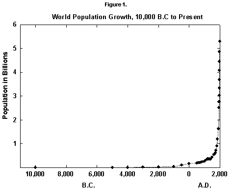
Fig. 1. World population growth, 10,000 B.C. to present. Sources of data: McEvedy and Jones [2] and United Nations [25].

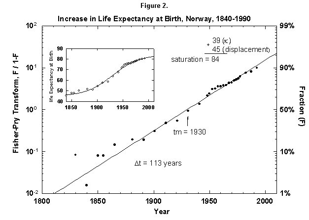
Fig. 2. Increase in life expectancy at birth, Norway, 1840-1990. A logistic curve fits the increase in life expectancy at birth. The logistic curve is displaced by 45 years, the life expectancy in 1845. As in most figures in this article, the logistic curve is plotted in both the traditional S-shaped form and in the Fisher-Pry transform. See Appendixes I and 2 for a description of the three parameters of the logistic model. Sources of data: United Nations [24] and Flora [16].

• 

Fig. 3. Increase in female life expectancy, by age, Norway, 1800-2050. Logistic curves fit the increase in life expectancy at various ages. For example, an 80-year-old person could be expected to live 6 more years in 1815 and 9 more years in 1975, an increase of life expectancy of 3 years. A logistic is fit to the points between 1815 and 1975. Source of data: Flora [16].

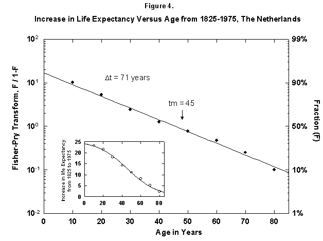
Fig. 4. Increase in life expectancy versus age, The Netherlands, 1825-1975. The figure shows that the increase In life expectancy is greater for the young than for the old, which implies an age limit. For example, a 10-year-old in 1975 had a life expectancy 24 years greater then in 1815. The actual life expectancy at each age is not shown on this graph. Source of data: Flora [16].

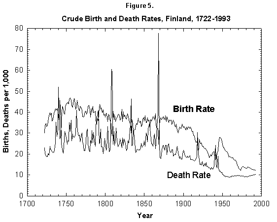
Fig. 5. Crude birth and death rates, Finland, 1722-1993. Birth and death rates have fallen by a factor of 4 since the 18^th century. The fluctuations from the mean also have decreased drastically. Sources of data: Lutz [17] and United Nations [24].

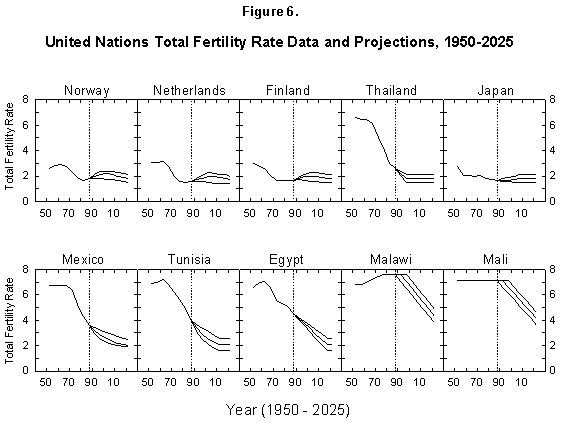
Fig. 6. United Nations total fertility rate data and projections, 1950-2025. The United Nations provides data and projections for 187 countries from 1950 to 2025. Source of data: United Nations [24].

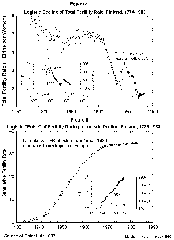
Fig. 7. Logistic decline of total fertility rate, Finland, 1776-1983. This figure fits a logistic curve to the decline in total fertility from a stable value in 1776 of 4.95 births per woman to the current value of 1.55 births per woman. The pulse of fertility in the 1940s and 1950s (squares) is modeled in Figure 8. Source of data: Lutz [17].

Fig. 8. Logistic “pulse” of fertility during a logistic decline, Finland, 1930-1983. This figure integrates the “pulse” of fertility evident in Figure 7 (the portion of the data plotted with squares instead of circles). The tbeoretical declining logistic curve was subtracted from this “bell-shaped” portion of the data, and the integral (cumulative sum) was then plotted and fit to a logistic curve to show the shape of the “babyboom” process. Source of data: Lutz [17].

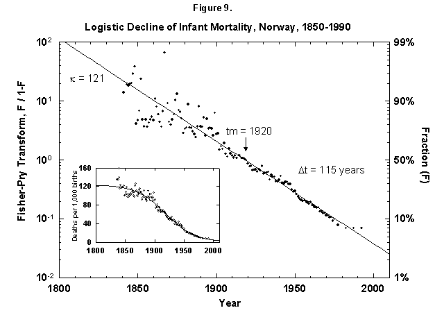
Fig. 9. Logistic decline of infant mortality, Norway, 1850-1990. The decline from 121 deaths per 1,000 infants born to 10 infants is dramatic and remarkably regular. The logistic was fit assuming a final goal of zero deaths, where the theoretical limit might be around 3 to 4, depending on advances in medical technology and screening procedures. Sources of data: Flora [46] and United Nations [24].

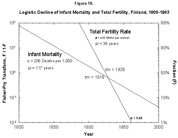
Fig. 10. Logistic declines of infant mortality and total fertility rate, Finland, 1800-1983. The Fisher-Pry transforms of the fitted logistics are plotted together for comparison. The data are not shown so as to ease comparison. Source of data: Lutz [17].

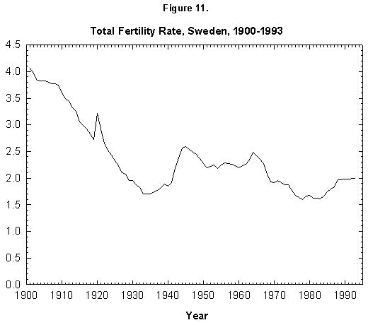
Fig. 11. Total fertility rate, Sweden, 1900-1993. Sources of data: Conseil de l’Europe [15] and United Nations [24].

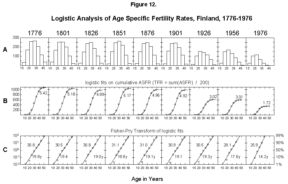
Fig. 12. Logistic analysis of age-specific fertility rates, Finland, 1776-1976. (A) Histograms of the age-specific fertility rates in 25-year intervals. (B) Integral (cumulative sum) of the bell-shaped histogram data, resulting in an S-shaped curve that is fitted with the three-parameter logistic. As explained in Appendix 3, the cumulative sum of the ASFR divided by 200 is equal to the total fertility rate (TFR). (C) Fisher-Pry transforms of the corresponding logistics (rendering them linear). Source of data: Lutz [17].

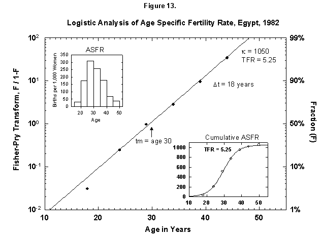
Fig. 13. Logistic analysis of age-specific fertility rates, Egypt, 1982. See Figure 12 and Appendix 3 for a description of the method of analysis used here. Source of data: United Nations [23].

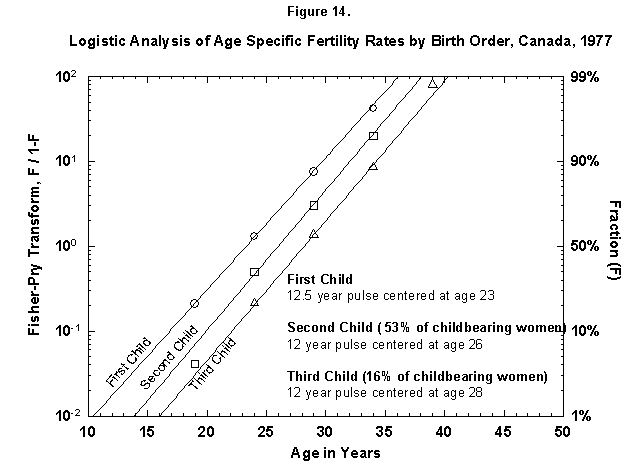
Fig. 14. Logistic analysis of age-specific fertility rates by birth order, Canada, 1977. The method of analysis used in this figure is similar to that used in Figure 12 and explained in Appendix 3, but here the fertility data are broken down further by the birth order, that is, first child, second child, and so on. The percentages refer to the number of women who go on to have more children (53% of Canadian childbearing women had a second child, but only 16% had a third child.) Source of data: United Nations [23].

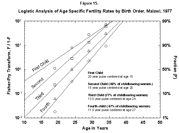
Fig. 15. Logistic analysis of age-specific fertility rates by birth order, Malawi, 1977. See Figure 14. Source of data: United Nations [23].

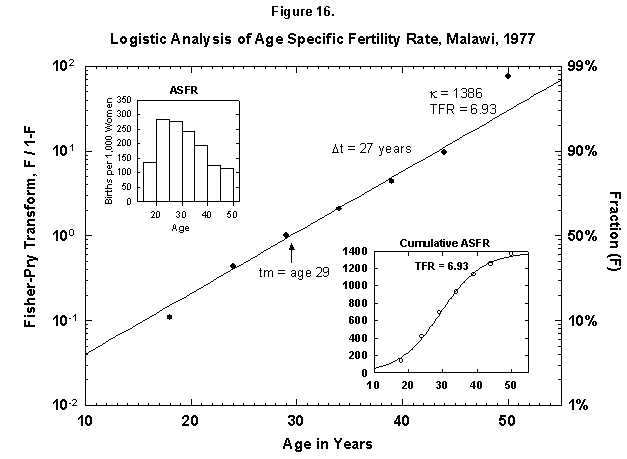
Fig. 16. Logistic analysis of age-specific fertility rates, Malawi, 1977. See Figure 12 and Appendix 3 for a description of the method of analysis used. Source of data: United Nations [23].

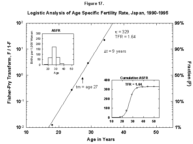
Fig. 17. Logistic analysis of age-specific fertility rates, Japan, 1990-95. See Figure 12 and Appendix 3 for a description of the method of analysis used. Source of data: United Nations [24].

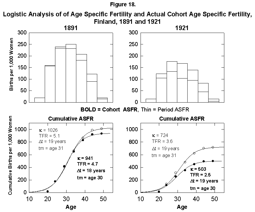
Fig. 18. Logistic analysis of age-specific fertility and actual cohort age-specific fertility, Finland, 1891 and 1921. Top: Histograms of both the ASFR and the Period ASFR, which follows the fertility rates of a 5-year cohort of women throughout their actual reproductive careers. Bottom: Corresponding logistics. PeriodASFR differ from the cohort ASFR when the fertility rates are rapidly changing, as shown by the 5-year age cohort from 1921 to 1961. Source of data: Lutz [17].

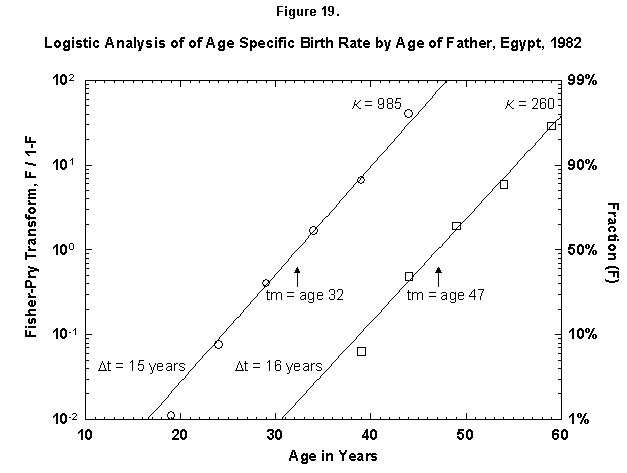
Fig. 19. Logistic analysis of age-specific birth rates by age of father, Egypt, 1982. This figure is similar to Figures 12-18 in that the cumulative ASFR is analyzed with logistics. However, this figure shows the cumulative ASFR by the age of the father as the sum of two logistic pulses. Source of data: United Nations [23].

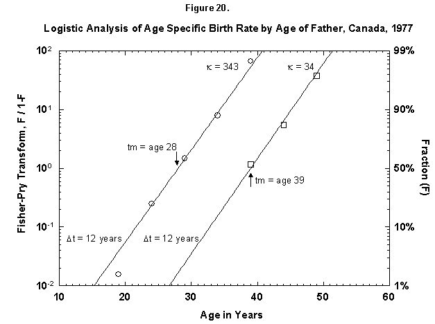
Fig. 20. Logistic analysis of age-specific birth rates by age of father, Canada, 1977. This figure shows the cumulative ASFR by the age of the father as the sum of two logistic pulses. Source of data: United Nations [23].

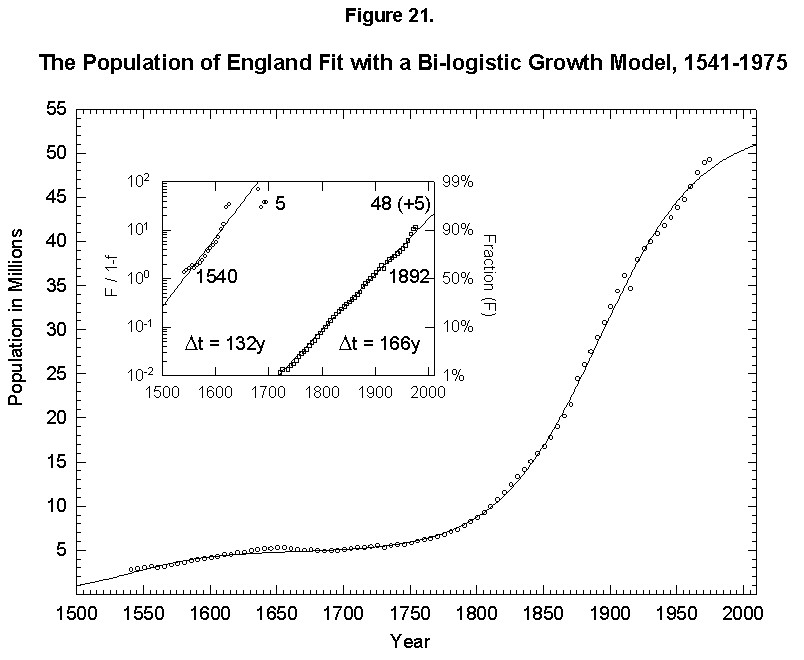
Fig. 21. The population of England fit with a bilogistic growth curve, 1541-1975. The sum of two logistics is used to analyze the population history of England. The first logistic curve has a 132-year characteristic growth time and a limit of 5 million and is centered in 1540. The second has a characteristic growth time of 166 years and a limit of 48 million and is centered in 1892. See Meyer [46] for a description of the bilogistic model. Sources of data: Wrigley [28] and Flora [46].

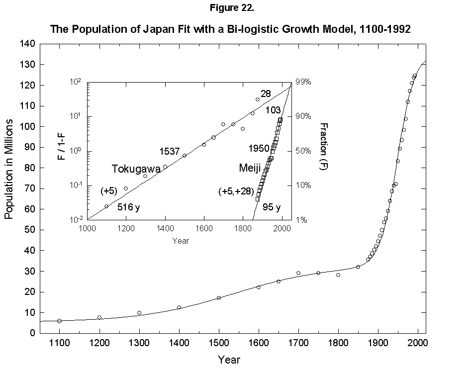
Fig. 22. The population of Japan fit with a bilogistic growth curve, 1100-1992. The sum of two logistics is used to analyze the population history of Japan. Adding on to an earlier base population of 5 million is a logistic with a 516-year characteristic growth time and a limit of 28 million centered in 1537. A second logistic curve with a 95-year characteristic growth time and a limit of 103 million centered in 1950 is added. See Meyer [46] for a description of the bilogistic model. Sources of data: Taeuber [21] and Tsuneta Yano Memorial Society [22].

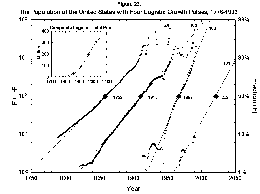
Fig. 23. The population of the United States with four logistic growth pulses, 1776-1993. The population of the United States is analyzed with the sum of four logistics centered on periods of rapid economic growth. The actual population is the sum of the logistics. In the inset the actual U.S. population data are fitted to a composite, or “superlogistic,” determined by the midpoints of the four component logistics. Sources of data: U.S. Bureau of the Census [26, 27].

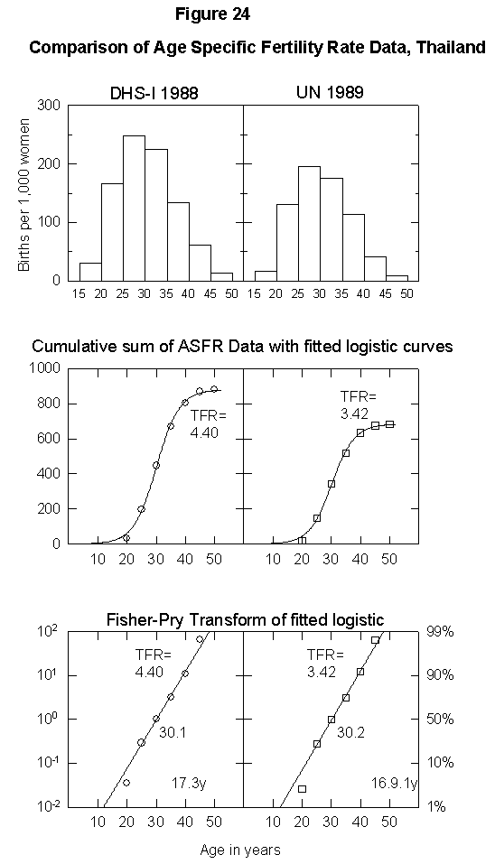
Appendix Fig. 1. Comparison of age-specific fertility rate data, Thailand. Left: Data from the Demographic and Health Survey (DHS). Right: UN data reported for the same year. Sources of data: United Nations [25] and Muhuri et al. [19].

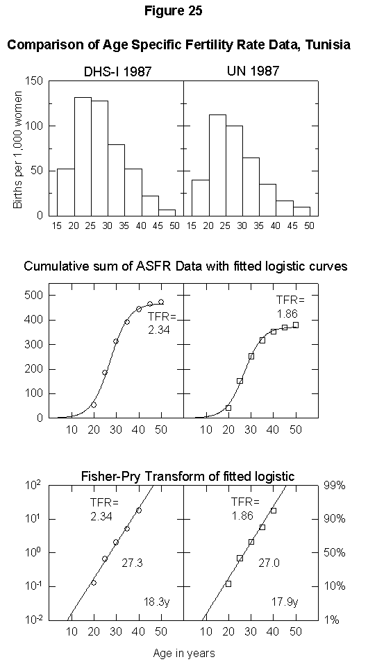
Appendix Fig. 2. Comparison of age-specific fertility rate data, Tunisia. Left: Data from the Demographic and Health Survey (DHS). Right: UN data reported for the same year. Sources of data: United Nations [25] and Muhuri et al. [19].References

I. Darwin, C., On the Origin of Species by Means of Natural Selection of the Preservation of Favoured Races in the Struggle for Life [1859], reprinted by Random House, New York, 1993.

2. McEvedy, C., and Jones, R., Atlas of World Population History, Penguin, New York, 1985.

3. von Foerster, H, Mora, M. P., and Amiot, L. W., Doomsday: Friday, 13 November, A.D. 2026, Science 132, 1291-1295 (1960).

4. Petersen, W., Population, 2nd ea., Macmillan, London, 1969, p. 333.

5. Keyfitz, N., Population: Facts and Methods of Demography, Freeman, San Francisco, 1971.

6. Keyfitz, N., Can Theory Improve Population Forecasts?, Report WP-82-39, IIASA, Laxenburg, Austria, May 1982.

7. Lutz, W., The Future Population of The World: What Can We Assume Today?, Earthscan Press, London, 1994.

8. Cohen, 1. E., How Many People Can the Earth Support?, Norton, New York, 1995.

9. Lee, R. D., and Tuljapurkar, S., Stochastic Population Forecasts for the United States: Beyond High, Medium, and Low, Journal of the American Statistical Association 89(428), 1175-1189 (1994).

10. United Nations, United Nations Demographic Yearbook, United Nations, New York, 1952.

11. United Nations, Long-Range World Population Projections: Two Centuries of Population Growth, 1950-2150, United Nations, New York, 1992.

12. Banks, R. B., Growth and Diffusion Phenomena: Mathematical Frameworks and Applications, Springer, Berlin, 1994.

13. Gruebler, A., and Nakicenovic, N., eds., Diffusion of Technologies and Social Behavior, Springer, Berlin, 1991.

14. Lotka, A. J., Elements of Physical Biology, Williams & Wilkins, Baltimore MD, 1924. Reprinted by Dover, New York, 1956.

15. Conseil de l’Europe, “La Fécondité des cohortes dans les états membres du conseil de l`Europe,” Etudes Démographiques 21, Strasbourg, 1990.

16. Flora, P., State, Economy, and Society in Western Europe, 1815-1975, St. James Press, Chicago, 1983.

17. Lutz, W., “Finnish Fertility Since 1722: Lessons from an Extended Decline,” The Population Research Institute at the Finnish Population and Family Welfare Federation, Helsinki, Finland, 1987.

18. Mitchell, B. R., European Historical Statistics, 1750-1975, 2nd rev. ea., Facts on File Publications, New York, 1981.

19. Muhuri, P. K., Blank, A. K., and Rutstein, S. O., Socioeconomic Differentials in Fertility, Demographic and Health Surveys Comparative Studies No. 13, Institute for Resource Development/Macro Systems, Inc., Columbia, MD, 1994.

20. Pressat, R., The Dictionary of Demography, Blackwell, Oxford, England, 1985.

21. Taeuber, 1. B., The Population History of Japan, Princeton University Press, Princeton, NJ, 1958.

22. Tsuneta Yano Memorial Society, NIPPON, A Charted Survey of Japan, Kokusei-Sha Corp., Tokyo, Japan, various years.

23. United Nations, 1986 Demographic Yearbook (Special Topic: Natality Statistics), United Nations, NewYork, 1988.

24. United Nations, World Population Prospects: The 1992 Revision, United Nations, New York, 1993.

25. United Nations, 1992 Demographic Yearbook (48^th Issue Special Topic: Fertility and Mortality Statistics), Population Division, New York, 1994.

26. U.S. Bureau of the Census, Statistical Abstract of the United States: 1994(114 ed.), United States Department of Commerce, Washington, DC, 1994.

27. U.S. Bureau of the Census, Historical Statistics of the United States: Colonial Times to 1970, United States Department of Commerce, Washington, DC, 1975.

28. Wrigley, E. A., and Schofield, R. S., The Population History of England, 1541-1871: A Reconstruction. Edward Arnold Ltd., London, 1981.

29. Marchetti, C., Society as a Learning System, Technological Forecasting and Social Change 18(3), 267-282 (1980).

30. Yashin, A. 1., and Iachine, 1., How Long Can Humans Live? Lower Bound for Biological Limit of Human Longevity Calculated from Danish Twin Data Using Correlated Frailty Model, Mechanisms of Ageing and Development 80, 147-169 (1995).

31. Eigen, M., Self-Organization of Matter and the Evaluation of Biological Macromolecules, Die Naturwissenschaften 10, 465ff (1971).

32. Hausfater, C., and Hrdy, S., eds., Infanticide: Comparative and Evolutionary Perspectives, Aldine, New York, 1984.

33. Hirschman, C., Why Fertility Changes, Annual Review of Sociology 20 203-233 (1994).

34. Galloway, P. R., Basic Patterns in Annual Variation in Fertility, Nuptiality, Mortality, and Prices in Pre-industrial Europe, Population Studies 42, 275-302 (1988).

35. T. W, and Population Reference Bureau Staff, World Population in Transition, Population Bulletin 41(2), Population Reference Bureau, Washington, DC, 1991.

36. Imhoff, A. E., Die gewonnen Jahre: Von der Zunahme unserer Lebenspanne seit dreihundert Jahren oder von der Notwendigkeit einer neuen Einstellung zu Leben und Sterben, C. H. Beck, Munich, 1981, p. 53.

37. Rose, L., Massacre of the Innocents: Infanticide in Great Britain, 1800-1939, Routledge & Kegan Paul London, 1986.

38. Harris, M., and Ross, E. B., Death, Sex, and Fertility: Population Regulation in Preindustrial and Developing Societies, New York, Columbia University Press, 1987.

39. Ahn, N., Measuring the Value of Children by Sex and Age Using a Dynamic Programming Model, Review of Economic Studies 62, 361-379 (1995).

40. Riddle, J. M., Contraception and Abortion from the Ancient World to the Renaissance, Cambridge University Press, Harvard, 1992.

41. Move to Stop Sex-Test Abortion, Nature 324, 202 (1986).

42. Dickemann, M., Female Infanticide, Reproduction Strategies, and Social Stratification: A Preliminary Model, m Evolutionary Biology and Human Social Behavior: An Anthropological Perspective, N. Chagnon and W. Irons, eds., Duxbury Press, North Scituate, MA, 1979 p. 328.

43. Keyfitz, N., How Secure Is Social Security?, Report WP-81-101, IIASA, Laxenburg, Austria, July 1981.

44. Le Play, M. F., La Réforme sociale en France, Henri Plon, Paris, 1864, chap. 2.

45. Marchetti, C., Action Curves and Clockwork Geniuses, in Windows on Creativity and Invention, J. G. Richardson, ea., Lomond, Mt. Airy, MD, 1988, pp. 25-38.

46. Meyer, P., Bi-Logistic Growth, Technological Forecasting and Social Change 47(1), 89-102 (1994).

47. Smith, D., and Keyfitz, N., eds., Mathematical Demography: Selected Papers, Springer, Berlin and New York, 1977, pp. 333-347.

48. Kingsland, S., The Refractory Model: The Logistic Curve and the History of Population Ecology, The Quarterly Review of Biology 57, 29-52 (1982).

49. Putnam, P. C., Energy in the Future, Van Nostrand, New York, 1953.

50. Meade, N., and Islam, T., Forecasting with Growth Curves: An Empirical Comparison, International Journal of Forecasting 11, 199-215 (1995).

Received August 23, 1995; revised January 15, 1996; accepted January 16, 1995