Definitions and notation

Consider the two-dimensional space in which our data set $D$ exists. If there are $m$ data points, then we define $D$ as

$$D = \{(t_1,d_1), \ldots ,(t_i,d_i), \ldots,(t_m,d_m)\}$$

where $t_i$ usually represents time, while $d_i$ represents the growing variable (e.g., number of organisms, percent of saturation).

Suppose we want to fit a logistic curve of $n$ components to the model. Then we will require $3n$ parameters, represented as a $n \times 3$ matrix $\bold P$, where the $i$th row describes the $i$th component:

$$\bold P = \left[ \begin{array}{ccc} \Delta t_1 & \kappa_1 & t_{m1} \\ & \vdots & \\ \Delta t_n & \kappa_n & t_{mn} \end{array} \right]$$

Thus a loglet can be alternatively specified by

$$\bold{N}(t, \bold P) = \sum_{i=1}^{n} \frac{\bold P_{i2}}{1 + \text{exp} \left[ {-\frac{\ln(81)}{\bold P_{i1}}}(t - \bold P_{i3}) \right] }$$

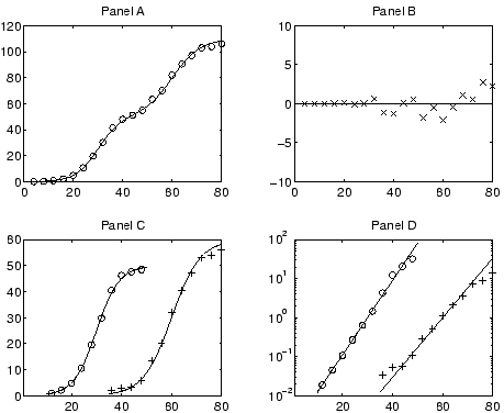
Figure 5A shows a hypothetical data set (the circles) and a fitted loglet with $n=2$ and

$$\bold P = \left[ \begin{array}{ccc} 20 & 50 & 30 \\ 25 & 60 & 60 \end{array} \right].$$

Gaussian noise was added to the data to dataset to show the residuals.

Figure 5: A hypothetical bi-logistic data set(A), the residuals of the fitted curve(B), and the decompositions in raw form (C) and with the Fisher-Pry transform applied (D).