Jason Yung, Perrin S. Meyer, and Jesse H. Ausubel
Program for the Human Environment
The Rockefeller University
New York, NY
July 1998
Trends commonly accelerate, reach a maximum speed, and then slow as they
approach some limit. After a sunflower seed germinates, the plant grows faster
and faster because each cell produces two, then the two produce two and so on.
But multiplication does not go on ad infinitum because the seed produces a
sunflower, not Jack's beanstalk; a sunflower stops before it reaches 20 feet.
The simplest description is the so-called logistic equation of three
parameters: the time of germination, the relative rate of growth and the limit.
Loglet Lab fits a single logistic equation to a series of observations through
time. It also displays the deviations of the observations from the logistic
equation, the result in linear form, and the rates of change.
Growth may slow and accelerate again. Imagine a drought or shortage of
fertilizer halts the sunflower's growth until rain or fertilizer starts a new
wave of growth toward the natural limit of sunflowers. Or imagine nuclear
testing multiplies as equipment and war scares increase; then scares recede and
testing slows, only to start a wave of testing toward another ceiling. As
"Loglet" contracts "logistic" and "wavelet," Loglet Lab fits
multiple logistic equations to such waves.
Competition causes a third variation of acceleration, slowing, and
reaching a limit as the competing substitute increases its market
share, and then declines as a new competitor becomes ascendant.
Consider the rise of long playing (LP) records of music, their
displacement by cassettes, and then the replacement of cassettes by
compact discs (CDs). Loglet Lab computes the market shares of each
competitor and fits their rise, leveling and fall with logistic
equations.
With this brief introduction you are now ready to enjoy
a tutorial that carries you through fitting a single logistic,
multiple logistics and the substitution of one competitor by another.
You can read about the mathematics in the online Help as well as in
the accompanying "Logistics
Primer."
We also append
a list of known bugs to this tutorial.
- Run A:\Setup.exe. This will run the InstallShield program.
- By default, Setup places files in C:\program files\ru-phe\loglet lab\. In
particular, the installation will install the following files which are
required to run Loglet Lab:
- Loglet Lab.exe: The actual Loglet Lab program
- Loglet Lab.hlp: on-line help file
- Vcf15.ocx: Formula One (spreadsheet) control
- Gallery\*.lgt: Data files
- Setup will also install or update the following files in the Windows system
directory if necessary:
- Axdist.exe
- Oleaut32.dll
- Mfc42.dll
- Olepro32.dll
- Msvcrt.dll
- Regsvr32.exe
- Stdole2.tlb
If older copies of any of the above files already exist on your computer,
registration of Vcfi5.ocx and Vcf15.ocx may fail; this is because the computer
has to restart before it uses the newer version. If this happens, you can
always enter the following commands using Run... in the Windows Start
Menu to register the controls manually:
Regsvr32 "C:\Program Files\RU-PHE\Loglet Lab\Vcf15.ocx"
- The installation should also have added Loglet Lab to the Start menu. You
can use this to start Loglet Lab.
- The first thing that you will see is the splash page, featuring a nifty logo
and a copyright notice. After 5 seconds, the splash page should go away,
leaving you with a blank document:
- As you can see, there are two panes: the Data View, where the
numerical data can be entered, viewed, and edited, and the Graph View,
where the data are graphically represented. Near the top of the window is a
toolbar, with buttons to execute the various commands in Loglet Lab. All of
the toolbar buttons have equivalent commands in the menus at the top of the
window.
- Click the mouse in the first (upper left) cell of the Data View grid. This
activates the grid; you should see a heavy black border around the first cell,
and a scroll bar should appear on the right side of the frame.
- The first column holds the time, and the second column holds the
corresponding values of y such as sales, height, or publications. The third
column holds the mask, which is used to withhold points from the fitting
process. Mathematically speaking, this corresponds to the "weight" of the data
point in the fitting process; for the most part, we will use all of points, so
the default is 1. Enter the following times and y-values in the first two
columns:
- Notice that as soon as you enter a new data point, it is plotted in the Graph
View. Only rows with both an x- and a y-value will be plotted.
- To fit a logistic to these data, click on the Fit Logistic button
 .
(Again, all of these commands are available on the Data menu.) This
will bring up the "Logistic Fitting Wizard" dialog box where you will
specify the number of logistic curves and the displacement of the logistic
curve from zero.
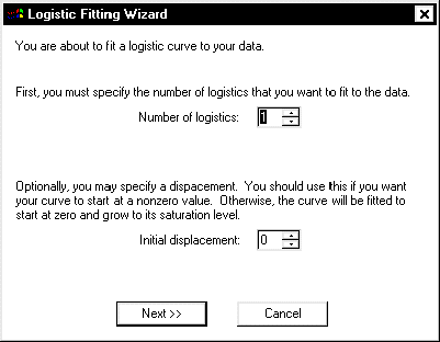
- You want to fit a single logistic to these data, so use the default "Number
of Logistics" of 1. You also should use the default "Initial Displacement" of
0. An example where it should be not be zero will be discussed later about
step 45. Click the "Next" button in the Wizard to proceed to the
"Specify Logistic Parameters" dialog box.
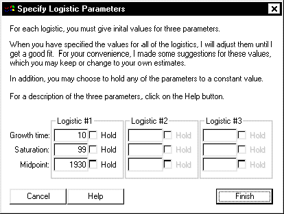
- Unlike linear regression, fitting a nonlinear equation requires initial
values for its coefficients. Using an iterative process, the parameters will
converge from these values to final values. For the first attempt to fit a
curve to these data, Loglet Lab will estimate values for each parameter; for
subsequent fits, it will provide the most recent set of parameters. You can
proceed with these values, or replace them with your own estimates. It is
recommended that you try Loglet Lab's estimates and then use your own estimates
based on the results of the first fit. For the three data which you currently
have, Loglet Lab's estimates will suffice.
- You can tell Loglet Lab not to change a particular parameter during the
process by clicking its corresponding "Hold" box; an "X" will appear in the
box. This is useful if external evidence supports a particular limit to the
saturation level or growth time; for instance, the growth of a bacteria culture
is limited by the size of the petri dish. However, for the purpose of fitting
a curve to these three data, you will not need to hold any of the
parameters.
- Because you are fitting a single logistic to these data, you do not have to
enter anything the other fields. (In fact, they should be deactivated by
Loglet Lab.) When you are satisfied with Loglet Lab's estimates or have
replaced them with ones you prefer, click OK.
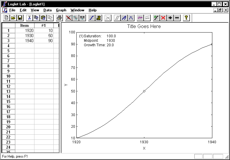
- Voila! Loglet Lab graces your screen with an elegant logistic, and places
the parameters of the fitted logistic in the upper-left corner. (If you hold
any of the parameters constant in the fit, they will be annotated with an
"(H)".)
- Once the glow of having fit your first logistic has subsided, you will want to
fit real data. Select Open from the File menu. We will be
delving into the "gallery" of examples that comes with Loglet Lab. Later you
can browse the gallery for sets that illustrate the range of logistic
processes.
- In the Open dialog box, double-click on sunflow.lgt to open the
sunflower data set. On some computers, the ".lgt" will not appear.
- Because many phenomena rise and level off, it is not obvious that you are
looking at the growth of a sunflower. To convey this, add a title and label
the axes on the graph. Click on the Edit Labels button
 to bring up the "Edit Labels" dialog.
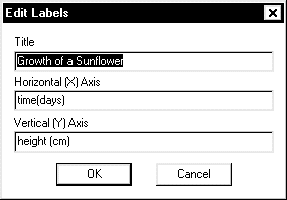
- In the Title field, enter "Growth of a Sunflower". For the X-axis,
enter "time (days)" and for the Y-axis, enter "height (cm)".
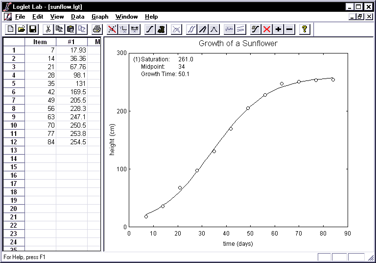
- Fit a logistic to the growth of a real sunflower as you did for the
fictitious three points in the preceding exercise. If all is well, a logistic
with Growth time=50, Saturation=261, and Midpoint=34 will
appear on your screen.
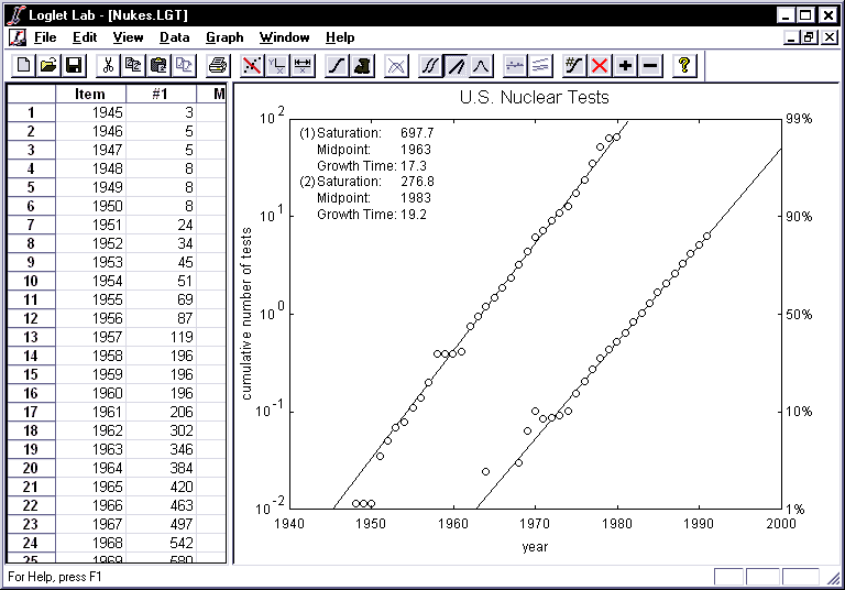
- A linear representation of the logistic and the data can provide a
different interpretation of the model. This can be obtained by applying the
Fisher-Pry transformation and plotting the transformed curve and data on a
semi-logarithmic scale. The transform is y' = F/(1-F)
where F is the ratio of y to the saturation level. This turns a
logistic curve into a straight line which shows growth as the percentage of the
saturation level. To apply the Fisher-Pry transformation, click on the
Fisher-Pry button
 .
Note that the y-axis has automatically changed to a logarithmic scale. To
toggle back to the graph of absolute y versus absolute time, click on
the Fisher-Pry button again.
- You will want to examine how fast as well as far the sunflower has grown.
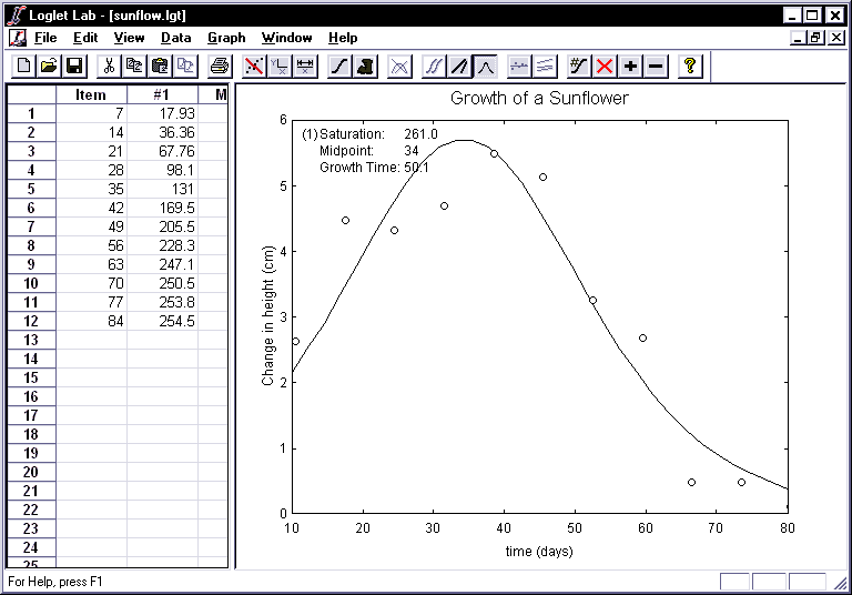
The rate of change of a logistic function is bell-shaped; click the Bell
Curves button
 to see the rise and fall of the rate of change. To toggle back to the graph of
absolute y versus absolute time, click on the Fisher-Pry button again.
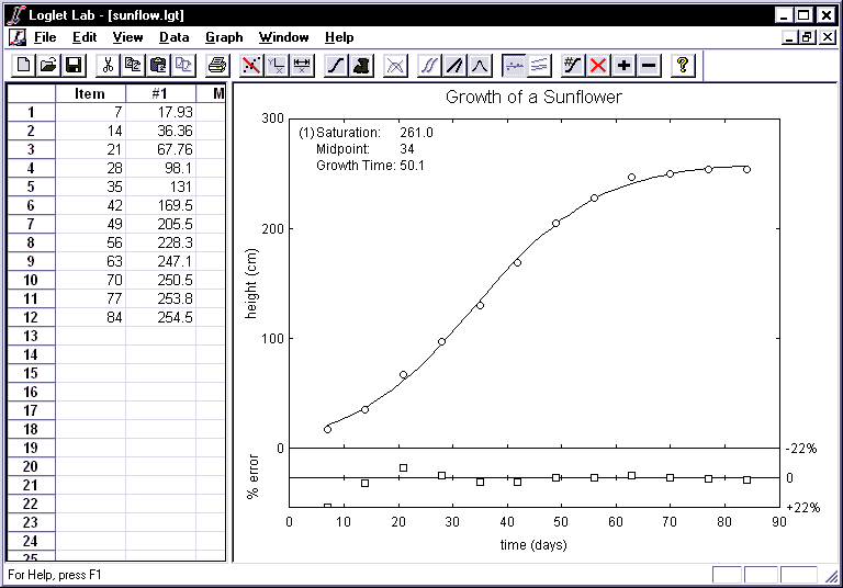
- You will also want to see how well this single logistic curve fits the
data. Clicking on the Hide/Show Residuals button
 displays the differences between the actual values and those predicted by the
logistic equation you have fitted. If the residuals are large or systematically
distributed, better fits are likely to be attainable, or perhaps the growth is
not logistic. (Section 5 of the Logistic Primer describes residuals in
detail.)
- The first time you click on the Hide/Show Residuals button, Loglet Lab
presents the error as a percentage of the actual value. The graph of percentage
errors is scaled to fit the maximum error. A second click shows the absolute
errors, the simple difference between actual and predicted values, which like
the graph of percentage errors is scaled to fit the maximum error. A third
click cycles back to the graph of absolute y versus absolute time.
- Now let's try a bi-logistic. Growth may slow and accelerate, as when a
drought slows the sunflower's growth until rain feeds new wave of growth
toward the natural limit of sunflowers. Or imagine nuclear testing multiplies
as equipment and war scares increase; then scares recede and testing slows,
only to start a wave of testing toward another ceiling. To see this, you will
now fit two logistic curves to the two waves of nuclear testing. Select
Open from the File menu, double-click on Nukes.lgt, and
the record of U.S. nuclear tests will appear in the data view.
- Click on the Fit Logistic button. This time you will want to fit
two logistics, so replace the '1' with a '2'. Because no nuclear tests
preceded 1945, leave 0 as the displacement. Click on the Next button to
specify the parameters for each logistic wave.
- Because you are fitting two logistics for these data, you will have
to specify six parameters, three for each logistic. Note that Loglet
Lab has activated the fields in the "Logistic #2" box in the "Specify
Logistic Parameters" dialog. Moreover, Loglet Lab has adjusted its
estimates to accommodate two logistics.
- Click OK to accept the parameters.
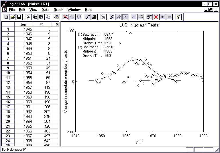
- Boom! A nice bi-logistic has just been fitted to the two waves of nuclear
testing.

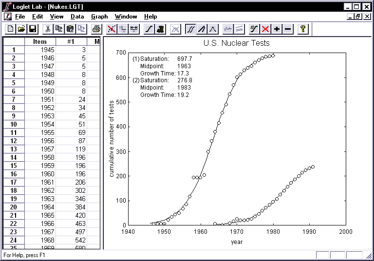
- A multi-logistic can be decomposed into logistic pulses to show the
discrete growth periods of each pulse. Moreover, there are several methods for
decomposition. To look at the decomposition in absolute numbers, click on the
Decompose into Components button
 .
The total saturation is 975 nuclear tests, of which 698 can be attributed to
the first wave of growth, and 277 to the second. By decomposing the logistic,
we can see each component rise to its respective limit, and the time span of
its effects.
- Clicking on the Fisher-Pry button displays the two linear transformations
of the components.
- Clicking on the Bell Curves button displays the rate of change of each
component. For your convenience, Loglet Lab uses a different marker to denote
the individual components. In this example, the first component is represented
by circles, and the second component is represented by diamonds. The y-axis
label now reads "change in cumulative number of nuclear tests".
- Admittedly, the discrete rate of change tends to look noisy compared to the
idealized model. Thus it may make sense to hide the data points and look at
just the fitted curve. To do this, click the Hide/Show Data Points
button
 .
.
- How precise is this fit? That is, how sensitive is this fit to
sampling error? Using a technique called the Bootstrap method, we can compute
a confidence interval for each of our parameters. For a detailed
description of the bootstrap, consult Section 4.3 of the Primer, which is
motivated by An Introduction to the Bootstrap by Bradley Efron and
Robert J. Tibshirani.
- Put simply, the bootstrap works as follows. First, a curve is fit to the
data as per the previous sections. Then a new set of data is synthesized based
on the residuals from the initial fit, and a curve is fitted to each of this
set. The process of synthesizing and refitting is repeated 200 times. This
gives us 200 values for each parameter, from which the mean and standard
deviation can be computed. To demonstrate the bootstrap method, reopen the
sunflower data and click on the Bootstrap button
 .
.
- To start the bootstrap, you have to fit a curve to the actual data. Thus
your first steps will be fit a curve as above. Then Loglet Lab will execute
the bootstrap. While the bootstrap is being executed, you will see a progress
bar which shows how many iterations have been executed. (Even on our 200MHz
Pentium Pro with 64MB RAM, this takes about 5-10 seconds, so be patient.)
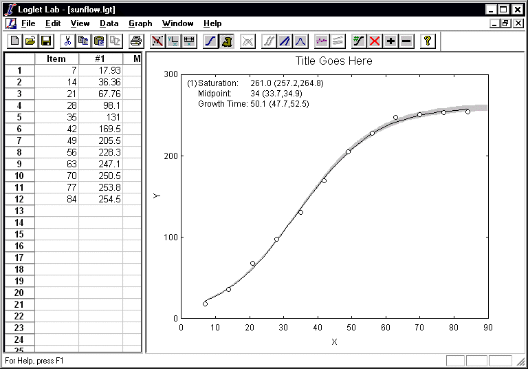
- When Loglet Lab is finished running the bootstrap, it will print the 90%
confidence interval (CI) for each parameter next to its respective value. A
gray region will be appear on the graph, showing the range of curves with
Saturation values within its 90% CI. Clicking on the Bootstrap button will
cycle through the different parameters to show how varying a particular
parameter affects the confidence region of a fit. (The parameter being varied
over its confidence interval is indicated in the lower right corner.)
- You can set the number of iterations and the level of confidence by
selecting Bootstrap Options from the Data menu. You can also the
seed for the random number generator for comparing with other fits.
- Be careful when using the bootstrap method for multi-logistic curves. This
is apparent when looking at the confidence region for Saturation, where error
increases as time increases, even after the curve has reached 99% saturation.
For such analyses, we recommend that you do an initial fit without the
bootstrap, and then run the bootstrap with the parameters held for one
logistic, i.e., vary the parameters for one logistic at a time.
- Including the years around 1959 when there was an extraordinary 4-year leap and
then hiatus in testing in our analysis may obscure the fit. Often it is
helpful to search first for fits using the "quiet" years of the data, when a
process appears to be unfolding without much disturbance such as war or
depression. Or, you might wish to exclude the years before or after 1971 to
examine one of the waves more closely. Loglet Lab lets you exclude data points
from the fitting process. First, click in the Data View to make sure it is
active. This is signified by the scroll bars and a heavy border surrounding a
cell.
- Scroll down until you can see 1969 through 1991 in the pane.
- Click on the "1971" cell. With the left button held down,
drag the mouse down to the "936" cell, selecting the data to be
excluded.
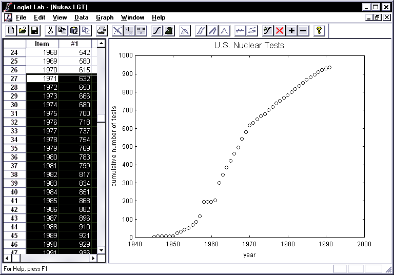
- Click on the Exclude Data button
 .
(Note that double-clicking on the region has the same effect.) The following
will tell you that the points you selected have been excluded:
- The area you selected should turn gray.
- The corresponding points will be plotted in red in the Graph View.
- The corresponding rows in the "Mask" column will be 0.
- Try fitting a single logistic to the pre-1971 data by clicking on the
Fit Logistic button.
- You must set the number of logistics to 1. Leave the displacement at 0 and
click on the Next button.
- Because we have excluded the last 20 years from the fit, Loglet Lab filters
them out and estimates appropriate parameters based on the data from the first
25 years. Click OK to fit the single logistic to the data.
- This should yield a single logistic with parameters: Growth time=18,
Saturation=734, and Midpoint=1964.
- Now look at the Fisher-Pry transform for this fit. You should hit the Plot
Data button each time you change views, because otherwise the excluded points
may not be correctly marked. Notice that several points that were excluded are
on the regression line; perhaps they should not have been excluded!
- Because data are often stored on spreadsheets or other external files, Loglet
Lab allows you to import files into the Data View. The next exercise imports
data from Excel. In this exercise, you will also see a case where you will
need to specify a nonzero displacement, as well as a loglet with three waves.
The file elements.xls in the gallery documents the discovery of
the elements. The data are years and the cumulative number of elements known
in that year. The discoveries appear to have come in three waves, probably
corresponding to new physical and chemical techniques and instruments.
- Select Import from the File menu to open the Import
Data "dialog box".
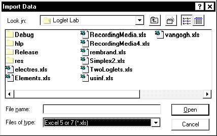
- At the bottom of this box is the Files of Type list box. Click on
the down arrow on the right end of the box, and select "Excel 5 or 7
(*.xls)" from the menu that drops down from the box. This will reveal all
Excel files in the directory.
- Select Elements.xls and click on the Open button. (You can
also double-click on the filename to achieve the same effect.) Loglet Lab
reads the Excel file and translates it into Data View.
- To fit three logistics to this data, enter 3 in "Number of
Logistics".
- Fourteen elements--for instance, gold--were known before 1735, the first
year of this series. Thus it makes sense to assume that growth of the number of
elements started at 14. Enter 14 as your "Initial Displacement," and click
Next.
- Unfortunately, for this data set, the estimates provided by Loglet Lab
won't work very well. They are based on an assumption that all three wavelets
are symmetric, which is inappropriate because the first wave of discoveries was
much longer in terms of the length of time and the amount of elements
discovered. With the rapid advancement of science near the turn of the
century, discoveries were more frequent in the subsequent waves. That said,
using the following parameters for each logistic should give you a suitable fit:
|
Logistic
#1
|
Logistic
#2
|
Logistic
#3
|
Growth
time
|
40
|
20
|
20
|
Saturation
|
40
|
30
|
20
|
Midpoint
|
1800
|
1890
|
1950
|
- Be sure to look at the decompositions for this logistic! Now you have seen
Loglet Lab's ability to fit logistics, from a simple rise and leveling to a
composite of several waves of growth.
- When importing from spreadsheets, Loglet Lab will fill in black spaces with
zeros. This will catastrophically affect any attempt to fit a curve to the
data. There are two ways to get around this. One is to interpolate values to
replace the zeros, which must be done by hand; another is to use the Remove
Data Points command to remove these rows. Should more data become
available, you can always use the Insert Data Points command to insert
more rows in your data.
- Using your mouse, select the cell(s) you wish to remove. (In our example,
we only select the y-values because Loglet Lab can figure out which pair of
values to remove; thus you can select cells in either or both columns and
achieve the same results.)
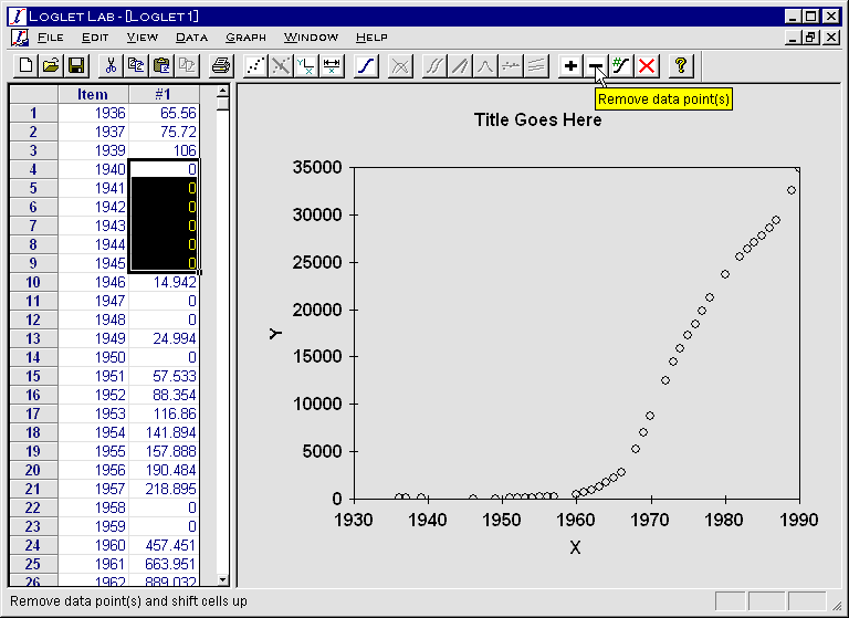
- Click on the Remove Data Points button
 .
The selected rows you selected will be deleted, and the cell(s) below it will
be shifted up.
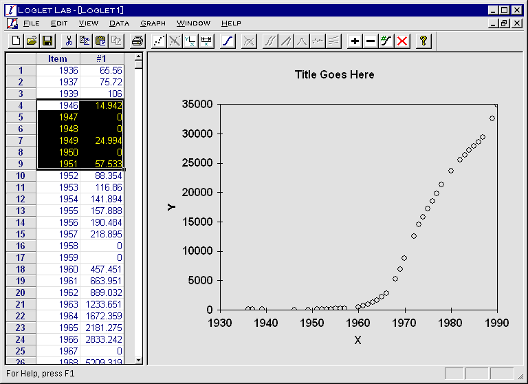
- The Insert Data Points command inserts rows in the column (or
rather, in a pair of columns). Using the mouse, select the range of rows where
you wish to insert data. If you want to insert 4 rows starting at row 17,
select rows 17 through 20.
- Click on the Insert Data Points button
 .
The rows you just selected and all the rows below them will be shifted down,
leaving blank rows in the selection area.
- You are now ready to see Loglet Lab's third capability: Analyzing the rise and
fall of competitors as one substitutes for another. We might analyze the
200-year displacement of packhorses with waves of wagons, canals, rails,
trucks, and recently airplanes. Instead of this long history that no one has
witnessed in a lifetime, you will analyze a history you may have witnessed: the
rise of long playing (LP) records, their displacement by cassettes, and then
the replacement of cassettes by compact discs (CDs). Loglet Lab computes the
market shares of each competitor and fits their rise, leveling, and fall with
logistic equations (You can read about the mathematics of logistic
substitution by clicking on Help and then Logistic Substitution
in the Help Index. It is also discussed in detail in Section 8 of the
Logistics Primer.)
- In addition to demonstrating logistic substitution, this exercise will show
how to paste data into Loglet Lab's Data View. Run Excel, and open
RecMedia.xls. This should be a 6x21 grid, the first pair of columns
being the year and annual sales of vinyl LPs, the middle pair the year and
sales of CDs, and the last pair for cassettes. Although the series of years in
all three pairs are identical in this file, they need not be; giving each
competitor its own series of years allows you to enter only the important years
for that competitor.
- In Excel, select the six columns containing the three pairs of years and
sales by clicking the first or upper left cell and dragging the mouse to the
lower right corner of the data.
- While you are still in Excel, click on the Copy button or
select Copy in the Edit menu.
- Go back to Loglet Lab, and open a new (empty) document.
- Click on the Number of Data Sets button
 .
This will bring up the following dialog box:
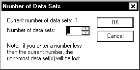
- For "Number of Data Sets," enter 3.
- Click on the first cell in the Data View pane, and make sure a heavy border
surrounds that cell.
- Click on the Paste Data button
 ,
or select Paste Data on the Edit menu.
- Click the Plot Data button to plot the sales in the Graph View for
each of the three competitors.
- To see the substitution of one competitor for another you need to convert
the sales of each into a percentage of the sales of all three. That is, you
need to replot the millions of sales into market shares. Click on the
Logistic Substitution button
 once to see the market shares, which have been plotted using the Fisher-Pry
transform.
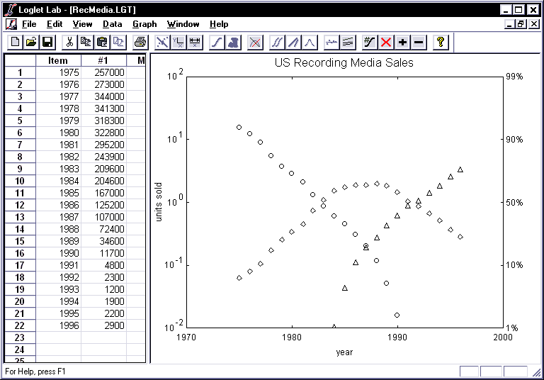
Because we are using the Fisher-Pry transformation, the linear portions of each
data series show the window in time or portion of its history that a logistic
equation logically represents.
- Next you need to fit a logistic to each competitor's record. Because LPs
only declined during this history, Loglet Lab fits a logistic to its decline
during 1975 to 1985, which the linear fall of the Fisher-Pry transform shows
was logistic. For cassettes, Loglet Lab will fit an equation to the logistic
portion of its rise during 1977 to 1985. Finally, Loglet Lab will fit an
equation to the logistic rise of CDs during 1988 to 1995. Clicking on the
Logistic Substitution button again opens the following dialog.
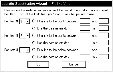
- Moving the dialog allows you to see the graph and the periods or windows
that you will specify. You will learn that Loglet Lab allows you to specify a
different order of substitution than the order of the columns in Data View.
Note the following regarding this data set:
- The first series, LPs, were already declining when this record began, and
their Fisher-Pry transforms from 1975 to 1985 line up well, displaying their
logistic behavior.
- The Fisher-Pry transforms of the third series, cassettes, rose linearly
from 1977 to 1985, so the market shares must have grown logistically during
that period.
- The Fisher-Pry transforms of the second series, CDs, rose logistically
from 1988 to 1995.
- Tell Loglet Lab the order of substitution by entering 1, 3 and 2 in "For
Item #" boxes on the left side of the dialog box.
- To fit the logistic curves, Loglet Lab must know the windows or time
intervals when a logistic equation is logical. We have already discussed these
above and they are visible in the graph of Fisher-Pry transforms. For Item #1,
LPs, enter "1975" and "1985" in the boxes to the right of "Fit a line between
____ and ____". For Item #3, cassettes, enter "1977" and "1985" after "Fit a
line between ____ and ____". For Item #2, CDs, enter "1988" and "1995" after
"Fit a line between ____ and ____".
- Make sure the order and intervals are correct. Then, click on the
Go button.
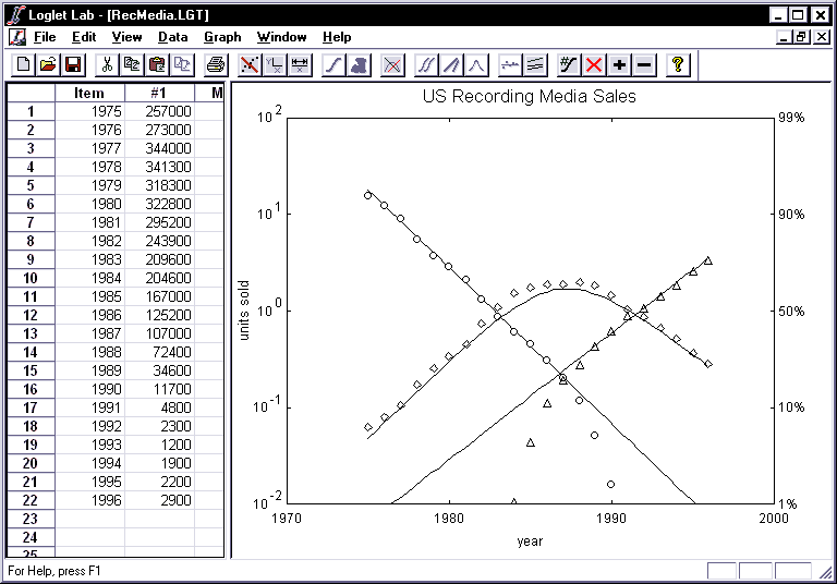
- The Graph View will show the linear representations of the three logistic
models. Three logistic equations now represent twenty years of rising and
falling sales of three competitors. Behavior is often irregular when a market
share is less than 5%; thus the model's line for the early years of the CD and
that for the later years of the LP are not as accurate.
- New technologies like the digital versatile disc (DVD) are poised to usurp the
CD's domination of recording media. Loglet Lab can visualize the impact of a
new technology on its competitors.
- First, you must tell Loglet Lab to accommodate the new, fourth technology.
Click on the Number of Data Sets button and enter 4.
- As you did for previously, click Logistic Substitution once to see the
market shares, and click it again to get the dialog box. The parameters from
the last fit should still be there, along with a new, fourth row. Since there
is no data for the DVD, you will have to tell Loglet Lab to synthesize a fourth
saturation curve for the new technology. For the new Item #4, click on
the radio button "Use the parameters dt =". This allows you to tell
Loglet Lab how well and quickly the new technology will compete. You specify
its competitiveness by dt, the time for it to rise from 10 to 90% of market
share; you specify how soon it will compete by tm, the midpoint of its rise.
We expect DVD's to grow at about the same rate as CD's, so try dt = 15 and tm =
2002.
- Click Go. The rise of the new competitor and consequent decline of
the third, CDs, will appear in Graph View.
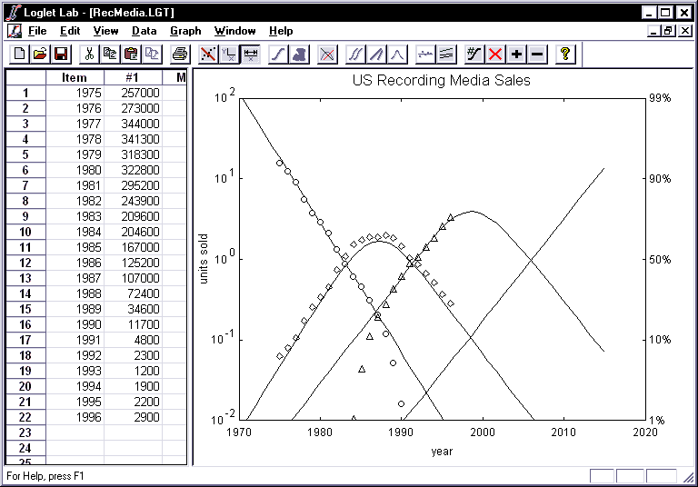
- Naturally, we would like to look beyond 1995. To extrapolate the history,
you can extend the x-axis. Click on the Extend Axes button
 .
This opens the following dialog:

- For the minimum, enter 1970, and for the maximum, enter 2015. Hit
OK to see the past and hypothetical future of recording sales in the
United States:
- If you want, you can go back and try different values for dt and tm. You
may also want to go back and try expanding the x-axis on other fitted data. In
particular, you can expand the right-side to see how the curves level off as
they approach limits.
- You can copy the data from the Data View to the Clipboard and paste them into
another spread sheet (e.g., Excel), word processor/text editor (e.g., Word,
emacs), or some other application (e.g., SigmaPlot). For your convenience, you
have access to the transformed data, decomposed data, fitted data points (i.e.,
the points Loglet Lab uses to plot the fitted curves), and the residuals.
- To get these points, select the view for which you which to copy data.
Then scroll the spreadsheet to find the columns which contain the data which
you wish to copy, and select them with your mouse.
- Click on the Copy Data button
 or select Copy Data on the Edit menu. This will copy the data to
the Clipboard. (For now, you cannot directly copy graphs onto the Clipboard,
at least not using Loglet Lab.)
- Finally, you can print any chart, by clicking on the Print button
or by selecting Print in the File menu. You may want to use
Print Preview to make sure the hard copy will suit your eyes.
- Applying exclusion to the generation of bell curves doesn't work quite
properly.
- For now, Loglet Lab can plot and fit logistic curves for only one series at
a time. That is, you are limited to one data series per plot. Thus the Fit
Logistic command is disabled when there is more than one data series in the
Data View. (Of course, if you have more than one data series in a document,
you can try to apply the logistic substitution model.)
- Some commands are handled slightly differently depending on whether the Data
View or the Graph View is active. A command may fail or misbehave because the
wrong pane is active. Be sure to let us know if this happens. Bugs aside,
all the commands are certain to work when the Data View is the active
pane.
- Do not be alarmed if, in the course of using Loglet Lab, the final
parameters turn out to be identical to the initial values. Loglet Lab is a
32-bit program, thus the final results are precise up to 16 digits, but they
are rounded off to the nearest integer. On the other hand, because the fitting
algorithm is iterative, it may be necessary to fit more than once before the
parameters converge sufficiently.
 .
(Again, all of these commands are available on the Data menu.) This
will bring up the "Logistic Fitting Wizard" dialog box where you will
specify the number of logistic curves and the displacement of the logistic
curve from zero.

 to bring up the "Edit Labels" dialog.

 .
Note that the y-axis has automatically changed to a logarithmic scale. To
toggle back to the graph of absolute y versus absolute time, click on
the Fisher-Pry button again.
  to see the rise and fall of the rate of change. To toggle back to the graph of
absolute y versus absolute time, click on the Fisher-Pry button again.

 displays the differences between the actual values and those predicted by the
logistic equation you have fitted. If the residuals are large or systematically
distributed, better fits are likely to be attainable, or perhaps the growth is
not logistic. (Section 5 of the Logistic Primer describes residuals in
detail.)

 .
The total saturation is 975 nuclear tests, of which 698 can be attributed to
the first wave of growth, and 277 to the second. By decomposing the logistic,
we can see each component rise to its respective limit, and the time span of
its effects.

 .
.

 .
.

 .
(Note that double-clicking on the region has the same effect.) The following
will tell you that the points you selected have been excluded:

 .
The selected rows you selected will be deleted, and the cell(s) below it will
be shifted up.
 .
The rows you just selected and all the rows below them will be shifted down,
leaving blank rows in the selection area.
 .
This will bring up the following dialog box:
 ,
or select Paste Data on the Edit menu.
 once to see the market shares, which have been plotted using the Fisher-Pry
transform.


 .
This opens the following dialog:

 or select Copy Data on the Edit menu. This will copy the data to
the Clipboard. (For now, you cannot directly copy graphs onto the Clipboard,
at least not using Loglet Lab.)